Why Fast Models are Destined to have a CPU Training Bottleneck
Contents
I was working on fixing the problem with a slow two-stage detector in my Smiling Robot by writing a faster deep detector from scratch. There’s ample research on fast detectors, but feature preprocessing for those is really complicated.
TensorFlow 2.0’s Dataset API has been pretty pleasant to use. It offers basic declarative API to
transform and shuffle feature vectors, and its batch balancing functionality is a godsend (I implemented batch
balancing without it, but now you can get that with 5 lines of code). It even
can parallelize your feature generation with
tf.dataset.map to however many CPU cores
you have.
However, do you want to generate this dataset “on the fly” as you train, or do you want to generate it ahead of time, and read it from disk? Here are your options:
- Saving training data to disk requires to pay an upfront cost in storage and training time (and writing some code), but you can run many many more iterations when finding the right model architecture and hyperparameters. And if you’re paying for GPU time, it’s better to utilize it at 100%.
- Generating data on the fly allows to change the data pipeline without paying a huge penalty. It works great when you’re just debugging your model and feature generation. However, if your data generation is slow, the training loop will be blocked on waiting for more data to come out of the feature generation pipeline.
What to choose? Interestingly (and perhaps surprisingly), if your goal is to build the model with fast inference time, you will have to choose the former: saving your data to disk. And even then, it might not be enough.
The Training Time Balance Equation
Imagine generating one feature vector takes $T_g$ seconds on CPU; you have C cores, your batch size is B, and your target model inference time is $T_i$ seconds. Now let’s assume the backwards pass takes as much time as the forward pass (this seems pretty reasonable given how backprop works), so each training iteration on one example would take $2T_i$. Then your pipeline will be bottlenecked by CPU if
Essentially, if the time to produce a new batch of features $T_g / C \cdot B$ is higher than how much it takes to make a forwards and backwards pass on a batch ($2T_i$), then at some point of time your model will be bottlenecked by CPU.
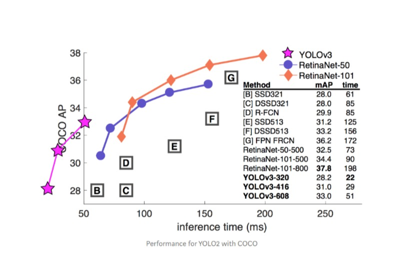
The effect is more pronounced if you’re specifically developing models with fast inference time. If your goal is to build an efficient model for say, a self-driving car, or a smiling robot that runs on a Raspberry Pi, your model’s inference time $T_i$ will be low because that’s exactly what you want it to be. This produces significant downward pressure onto the feature generation time.
So I wrote a quick-and-dirty timer for my training loop. The time to load and preprocess one feature turned out to be 0.028 seconds; I have 4 cores, and the training loop iteration takes 0.0104 seconds for a 32 batch. Let’s put the numbers into the equation:
So it seems, my GPU will spend $\frac{0.224}{0.224 + 0.010} = 96%$ of time waiting for new data, so the
utilization will be only 4%. This exactly matches what nvidia-smi says 😬.
Will buffering help?
Even if you add a buffer (via shuffle or prefetch), this buffer will be
eventually depleted before the training finishes. Buffering takes time, and the more you want to postpone
the buffer depletion by making a larger buffer, the more prefetching the buffer will take, and this equation
will never balance the way you intend. Think about it this way: the total time to run the training loop is
the max of these two timings:
- time to do forward and backward pass on each element in the dataset
- time to generate a feature vector on each element in the dataset (regardless of whether the element goes into the buffer when prefetching or when training)
Each of these is the Balance equation discussed above but multiplied by the dataset size. The equation doesn’t have a term for the buffer size; therefore it doesn’t matter.
Why use buffers then? Buffering helps to combat variance in the training data acquisition time (e.g. when reading from a volatile remote disk: read more when reads are fast, so you can read less when the reads are slow without losing progress). It does not help speed up training time averaged over large periods of time.
How to save to disk
So it’s completely sensible to start with a pipeline on the fly, iron out the data until you’re confident that the feature vectors are correct, and then to save the large dataset to disk. Saving the data to disk takes only very few lines of code.
I tried it by using tf.Dataset.shard in combination with this guide, but for some
reason it works very slow.
def _bytes_feature(value):
    """Returns a bytes_list from a string / byte."""
    if isinstance(value, type(tf.constant(0))):
        value = value.numpy() # BytesList won't unpack a string from an EagerTensor.
    return tf.train.Feature(bytes_list=tf.train.BytesList(value=[value]))

def _float_list_feature(values):
    """Returns a float_list from a float / double."""
    return tf.train.Feature(float_list=tf.train.FloatList(value=values))

def serialize_example(entry_key, entry_img):
    example_proto = tf.train.Example(features=tf.train.Features(feature={
        'key': _bytes_feature(entry_key),
        'img': _float_list_feature(entry_img)}))
    return example_proto.SerializeToString()

NUM_SHARDS = 10
for i in range(NUM_SHARDS):
    shard = self.train_dataset.shard(NUM_SHARDS, i)
    def tf_serialize_example(entry):
        tf_string = tf.py_function(
            serialize_example,
            (entry['key'],
             # tf.Example only supports flat arrays
             tf.reshape(entry['img'], (-1,))),
            tf.string)
        return tf.reshape(tf_string, ()) # The result is a scalar

    writer = tf.data.experimental.TFRecordWriter('sharded-dataset/shard-{}.tfrecords'.format(i))
    writer.write(shard.map(tf_serialize_example))
Well, I’ll debug this in the follow up posts.
