“What is the gradient of numpy broadcasting?” I was wondering the other night. It’s almost midnight, my brain is tired, and I got a bit stuck.

In short…

In numpy, broadcasting is adding a one-dimentional vector b2 to a 2-D matrix X, which implicitly adds b2 to every row of X.

To compute the derivative of the result over b2 (let’s call it g), we rewrite the expression as matrix multiplication. Here, B2 is a matrix of shape (M,1), which is just b2 with one extra axis, and $1^{B\times 1}$ is the broadcasting matrix:

$$X+b_2 = X + 1^{B\times 1}B_2^\top$$

In order to backpropagate the upstream gradient $G$, it gets multiplied by the transposition of the broadcasting matrix:

$$g^\top = \frac{\partial L}{\partial h_2} = 1^{1\times B} G$$

Effectively, $1^{1\times B}$ acts as a summator along the first axis ($g_k = \sum_{i=1}^B G_{i, k}$), which can be expressed as

Let’s explore how to get there in three different ways: the intuitive, the “compact form” and the “full form” tensor derivatives. But first, how did this even come about?

Midnight homework

Back then, I had just started my CS231n course studies as part of the Stanford SCPD certificate program. CS231n “Convolutional Neural Networks for Visual Recognition” is a great “starter” course if you study Deep Learning. We had to learn the basics and to manually implement and test quite a few backpropagation algoritms for simple network layers. I’ll write a more in-depth overview later.

Importantly, we got to really understand vector operations at a really low level, and we had to use a general purpose math library numpy as oppsoed to Deep Learning-specific Tensorflow or Pytorch.

Broadcasting in a Fully-Connected Layer

When I just started CS231n, I was used to that framework-level thinking about deep learning algorithms, and it took a bit of effort to shake it off. When implementing a two-layer fully-connected neural network using numpy, you add bias vector to the input batch multiplied by the weight matrix:

Here:

• X1 is a matrix of shape (B, N) where B is the batch size, and N the number of outputs from the first hidden layer.
• W2 of shape (N, M) where M is the number of outputs from the second hidden layer;
• b2 is the bias vector of shape (M).
• h2 of shape (B, M) is the output of the layer for each example in the batch.

But wait. The result of matrix multiplication X1.dot(W2) is of shape (B, M) so how can you add a vector of shape (M) to this? In numpy, as well as in our lecture notes, that’s called “broadcasting” and it’s a convenient method of working with batches of data. The code above essentially means “add b2 to every row of X1.dot(W2)” Our lecture notes told us to “use broadcasting” and I did. Neat.

Later, I was implementing backprop and for that, I needed to know the derivative of $\frac{\partial h_2}{\partial b_2}$. That’s when I got confused. What is the gradient of that “broadcasting”?

Intuitive derivation

We can ask a simpler question instead: how does $b_2$ contribute to the eventual loss $L$? Since it independently affects each example in the batch (and this means the impact onto each batch needs to be summed), we could simply compute the gradient of each example, and then sum the results along the batch axis. Tthat seemed too inventive to me at the time. Is there a more “mechanical” way to approach the task?

Broadcasting as matrix multiplication

To answer that, let’s think how to represent broadcasting without knowing that we operate in batches. Apparently, something happens to that b2 vector before it’s added to the product $X_1W_2$ , some function f is applied:

$$h_2 = X_1 W_2 + f(b_2)$$

In order for the addition to make sense, f should produce a matrix of shape (B, M) out of a vector of shape (M), such that each row of $f(b_2)$ equals $b_2$. Could it be matrix multiplication?

Indeed, if $f(b_2) = Zb_2^\top$, then Z is a matrix of shape (B, 1), and we can consider $b_2$ a matrix of shape (M, 1) (let’s actually start calling it $B_2$ since a one-column matrix and a vector are two different things). It makes sense if Z is simply a vector of ones (as in np.ones((1, B))):

$$f(b_2) = 1^{B \times 1} B_2^\top$$

So, the expression for $h_2$ becomes something more manageable:

$$h_2 = X_1 W_2 + 1^{B\times 1}B_2^\top$$

My first instinct was to try to define $\frac{\partial h_2}{\partial B_2}$. As I later learned, that’s not the most effective way: it only makes sense when operating on “full form” derivatives I’ll describe below. Instead of directly computing the “gradient of broadcasting”, we use it in backpropagation from the upstream gradient $G$:

$$\frac{\partial L}{\partial b_2} = \left(\frac{\partial L}{\partial B_2^\top}\right)^\top = \left(\underbrace{\frac{\partial L}{\partial h_2}}_{= G^\top} \frac{\partial h_2}{\partial B_2^\top}\right)^\top = \left(\frac{\partial f(B_2^\top)}{\partial B_2^\top}\right)^\top G = \left(1^{B \times 1}\right)^\top G = 1^{1 \times B}G$$

This is essentially the gradient of the broadcasting applied via the chain rule.

What does the expressions of $1^{1 \times B}G$ mean? If you look at the per-component layout of it, this expression effectively calculates the sum along the batch axis of the right-hand side matrix. Yep, the transposed “broadcasting” matrix becomes the summation matrix, and the end result will be:

$$g_k = \sum_{i=1}^{B}G_{i,k}$$

Compact and Full forms of tensor derivatives

Wait, why is $\frac{\partial L}{\partial h_2}=G^\top$ rather than $G$ ? And why did we end up with a matrix of shape (1, M) instead of the desired (M, 1)? Where all these transposition come from? Well, that’s because we’ve actually been using the “compact form” instead of the “full form” of tensor derivatives.

Yep, the way we usually operate with tensor derivatives, is by using the “compact form”, that omits quite a few zeros. You can read a great overview of this here in the CS231n lecture notes.

The actual “full” Jacobian of two matrices $\frac{\partial \mathbf{A}}{\partial \mathbf{B}}$ would be a four-dimensional array with the shape equivalent to $(a_1, a_2, b_2, b_1)$ (where $A \sim (a_1, a_2)$ and $B\sim(b_1, b_2)$–we’re using $\sim$ for “is of shape” here). However, in deep neural network calculus, one of these dimensions is usually a batch dimention. And batches are independent from one another. So most of the elements in the “full Jacobian” would be 0 (read more here). That’s why everyone uses a compact notation to only list the elements that matter. This requires you to be inventive and “get it”. But for me to “get it” I had to write it out in the full form.

$$\frac{\partial h_2}{\partial b_2} \sim (B, M, M) = (1^{B} \otimes I^{M\times M})$$

you can see how most elements of this matrix (let’s call it $M$) are indeed zeros, except that $M_{i, j, k}=1$ when $j=k$. In fact it only has M nonzero elements. This is consistent with that the “compact form” of $\frac{\partial \cdot}{\partial \mathbf{X}}$ is usually assumed to take shape of $\mathbf{X}$ itself. Compare the “full form”:

$$G_{full} = \left[\frac{\partial L}{\partial h_2}\right]_{full} \sim (1, M, B) $$

with the “compact form” we’re used to:

$$G = \left[\frac{\partial L}{\partial h_2}\right]_{compact} \sim (B, M) $$

Except for that extra axis, $G = G^\top_{full}$; that’s where the transposition comes from.

Overall, one can indeed operate the “full” derivatives in a more algorithmic way, but sadly that would increase the number of dimensions and require way more computation than the compact form.

I need to learn a bit more about how to represent derivatives with tensors and their product before trying to write out the full form for the expression above. I’ll update my post with this when I do: getting outer product for tensors with derivatives isn’t straightforward.

Perhaps there’s a way to both keep it “mechanised” and also simplify these expressions–let me know in the comments!

Driving on a highway is like picking stocks. There are multiple lanes, and as we established earlier, one of them is just faster than the others. Drivers take notice; they move into the lane just like the stock market players “move into” the stock of a promising company, buying its shares.

Then, the same thing happens as in the stock market: as more cars occupy the lane, it becomes more congested, and it slows down. The lane is no longer “profitable”, and other lanes start to outpace it. Recall the passive investment wisdom: no matter how hard you try, you will still move with the average speed of the flow (or, likely, worse). Unless you possess uncanny talent, or can see the future, or have insider knowledge, you have no advantage. On a freeway, talent won’t help, and as for seeing the future: you barely see behind that truck just ahead.

But I do have some insider knowledge for you. How come some commuters drone it out for 15 minutes in bumper-to-bumper traffic and those few “in the know” zoom past them and beat them to the next exit? Read on–or skip to the solution.

Enter the intersection of Highway 101 and Highway 92

Or, rather, enter the gigantic southbound traffic jam that “happens” there every single weekday, from 6.30am to 10am. The jam is so reliable that some atomic clocks use it as a backup time sync mechanism.

What happens there is simple. Three (!!!) different streams of traffic merge into this already clogged 4-lane highway: local 19th Ave, eastbound Highway 92, and westbound Highway 92, all full of techies anxious to make it to their 10am standup meeting. (Note that I might have mixed up the order of the on-ramps, but it’s not important for our purposes.)

The small outlet onto 92 doesn’t help as few people travel in that direction during peak hours. Or… does it?

If you’ve been a diligent student of traffic laws in the last several posts, you can see what’s happening here. The interchange is an interplay between four traffic situations:

1. right exit reducing the amount of traffic in the right lanes,
2. a slowdown at a merge that is causing the blockage in the right lanes.
3. “friction” that “carries over” the slowdown from the right lanes to the left lanes.
4. faster left lane getting backed up before the blockage.

We know from Traffic II that if there’s a blockage affecting all lanes, then the left (the faster) lane will be backed up more (this is pattern (4)):

(Here, the green circles mean “free flow”, the yellow “mild congestion, and the red “severe congestion”.)

What causes the blockage in the left lanes? It’s the friction from the blockage in the right lanes. What causes that? The three freaking merges that dump San Mateo and East Bay commuters onto 101.

So the traffic jam unfolds the same way every day: patterns (1) and (2) make the right lanes more congested, (3) carries over the slowdown from the right lanes to the left, and (4) causes the slowdown in the right lanes way way before the interchange. Here’s what the traffic looks like there:

The optimal strategy

So how do you beat the rat race? You got it: drive in the rightmost lane, and then merge left five times.

Indeed, in a simple two-lane case, the best way to traverse the blockage at the merge is to merge right just before the merge:

So when we apply this rule to the overall situation at the interchange, this would be the optimal strategy:

This doesn’t seem like much, but that’s because this model is very compressed. If we zoom out, the traffic would instead look like this:

It’s not easy and it is a bit stressful. Most prefer to just stay in the lane and relax, but if you want to get ahead in life, you gotta put some work in. Merging is tight: commuters do not appreciate the “freeloaders”, but it’s easier than it seems, just like the prior research shows.

A common mistake is to merge too early. Yes, I know you want to be conservative; yes, I know it’s hard to patiently watch that traffic slows down ahead of you; you want to react, you want to merge left, away from the impeding congestion… This is a mistake. If you’re in the right lane on 101, merge under the bridge, not before! Exercise patience. You’re the traffic tiger next to a flock of antelopes. Wait.

Another trick, employed by some shuttle bus drivers is to exit the freeway and immediately enter it. However, this involves a traffic light, and in my experience it’s not as fast as five merges (but if you’re driving a bus, merging is indeed more complicated).

Appendix

If you’re curious, I’ve filmed two videos of this interection.

Approach from Highway 101. Notice how three traffic lanes are merging into 101, and how motorists are merging leftwards. Before the overpass, the left lanes are more congested, and the traffic in the right lanes moves faster. However, as the camera approaches the overpass, left lanes pick up speed while the right lanes come to a standstil.

Approach from Highway 92. This time, we are merging into the right lanes that stall. Note how somewhat small amount of traffic coming off of Hwy 92 comes to a disproportinally slow merge at Hwy 101. You can also notice, at the time of merge that the left lanes are moving way faster than the merging lanes.

(Also some dude confused the shoulder with an extra lane… Oh if only!)

***

This concludes the traffic series. I originally wanted to write some simulations, but I realized there’s already a large body of work.

If you’re reading from outside of the US, you might be puzzled by what happens. In California, unlike on the East Coast or in Europe, drivers do not have a culture of staying in the right lane and using left lanes to pass only. Everyone basically drives wherever they want.

My old CPU was up for an upgrade (I’ve had it for 5 years), so I’ve built a new one. And since I’ve been studying Machine Learning, I needed way more computing power than I had.

When overclocking my system, I “de-lid” (“de-lidded”?) my CPU, replaced the thermal paste, upgraded to liquid cooling… What did I gain? Well, I have no freaking clue since I did not measure performance before statring. 🤦 Worst mistake ever. Don’t repeat it.

What is my setup?

• nVidia RTX 2080 Ti. nVidia GPUs are essential for machine learning these days, so I got an RTX 2080 Ti from EVGA (this one works great and will last me through the end of my studies).

• Core i7-9700k, a 8-core 4.6 GHz “gaming” CPU. For NLP deep learning, a GPU-powered machine learning algorithm will likely not use many CPU cores; instead 1 core will be used a lot. That informed the choice of CPU, and Intel’s Core i7-9700k which reportedly had best-in-class single-core performance.

  I later learned that multi-core performance is essential for ML models with complex input data (such as images). The CPU / GPU tradeoff heavily depends on the model and the data transforms you’re working with. If I don’t know anything about the model, I’d probably optimize towards multicore performace rather than single-core performance, and would go with a Threaripper.

For a short period of time, I’ve got the most advanced consumer CPU setup… The RTX demos and “Metro: Exodus” game hame look amazing… and ironically I don’t have any time to play them. 🤓

De-lidding Core i7-9700k

When researching CPUs, I found about “de-lidding”: “opening up” the CPU itself to replace the internal thermal compound with something better. Some Intel CPUs, they say, shipped with shitty stock thermal paste that wasn’t very efficient at heat transfer.

Core i7-9700k, however, ships with some sort of a metallic solder. How do I know that? Because I opened it up :-)

De-lidding was a well-established, well-documented, and well-researched procedure for older CPUs. There are even tools like “Delid die-mate” available to make it easier. My CPU was newer, so there was scant evidence, and most of it was recommending against de-lidding “for most users”, e.g. this video.

But I still did it, and the worst part, I don’t even know if it made any difference because I didn’t measure earlier. I have excuses: I was busy with school and I didn’t have time to measure anyway (“But you still had time to assemble a new PC, asshole!” says the voice in my head.)

Yes, my benchmark scores are through the roof, but they should’ve been through the roof to begin with.

Currently, I run my system at the following (“limiter” is why I didn’t OC it further):

* For some reason, the manufacturer website lists base core clock as 1635, but my benchmarking software as 1935. I’d trust the software. By the way, stock temp on my GPU was 66C under load.

I used Specy to measure the temperature, Precision X1 to overclock the GPU, Intel’s shitty-looking tool for the CPU. I used Unigine and 3DMark benchmarks to load the GPU, and CPU-Z to load the CPU.

What did I learn?

CPU cooler matters

CPU cooler matters, and matters a lot. I initially thought that I screwed the CPU up by de-lidding. The temperatures under load were up to 92C (!!!) That’s too much. Various overclocking forums recommend keeping an overclocked modern Intel CPU in the 60-s.

Replacing the basic cooler with a 240mm liquid cooling solution from Corsair helped.

That being said, I ran that CPU in the 80-85C range for days at a time (while training neural networks), and everything turned out fine. I could’ve just been lucky though.

Liquid cooling takes up space

Turns out, there’s not enough space in my computer case for the 240mm liquid cooling heatsink and the fans. My case is “only” 18 inches tall; I guess I’m up for an unexpected upgrade. My CPU looks like it “vomited” a radiator.

Building PCs is tedious

It was exciting the first time, when I was a 12 year old boy. Today, turning a million screws seems no better than assembling an IKEA drawer set. Getting best performance by tyning overclocking “hyperparameters” and then putting the results in a spreadsheet looks way too much like work or school.

De-lidding in more details

Here’s what de-lidding looks like. You’ll need the tools:

• der8auer Delid Die Mate 2 to remove the lid.
• Cardboard knife / razor / small kitchen knife to clean out the solder.
• Paper towels.
• really good “liquid metal” thermal compound because if not this, then why bother? Buy at least 2-3, because 1 pack is literally for 1 application, so if you screw it up (and the first time you will) you’ll need more.
• Medical tape or some other non-sticky tape (like a painter’s tape) to protect circuitry from liquid metal.
• A set of very fine sandpaper, 2000-3000 grit. This is to remove the solder and excess liquid metal when you screw up. You can skip this if you’re very patient and careful with sharp instruments.
• Silicone glue that can withstand heat and can glue metal (the CPU heatsink) back to the fiberglass CPU base (some say it’s optional tho).
• It’s best if your toenails are due for a trim, as toenails is the best tool for Step 3. (You can also use a non-sharp metal object or a credit card).

Step 1: Plug the untampered CPU in, and measure

Measure your performance first. You will spend hours assembling (took me 2 hours), delidding (4 hours), and then overclocking (5 hours) your PC; spend 20 minutes testing your assembled PC first. Use this:

• CPU-Z has a cpu load-test.
• Specy will show you a temperature graph (click on those green squares).
• Precision X1 will show GPU graphs (other use Afterburner)
• Even the free version of 3DMark will save your results online so you don’t have to write them down.

Step 2: Remove the lid!

Take the CPU out, clean up the thermal paste from it (you have it on because you measured first, remember?). Now use the Die-Mate tool as instructed in the manual, or watch it on youtube.

You’ll find that the lid covers literally nothing special. Just another black box.

Step 3: Clean out the thermal compound.

No, don’t use your toenails yet. That’s where you take out your exacto knife or a razor, and slowly and patiently scrub it out. That’s where you also understand that this whole thing is a waste of time, and you wish you hadn’t done it. Too late.

Once you’ve removed most of it, use fine (3000 grit or more) sandpaper to clean out the rest.

If your’re re-doing your prior work and scrubbing out liquid metal, be very careful! Do step 5 first (add tape), and then wipe it out with a paper towel. Be generous and never swipe the same side of the towel again: liquid metal will go right back.

Step 4: Clean out the silicon glue using your toenails or a non-sharp object

Toenails will just work, and a knife might damage the small metal components under it. Credit cards, or non-sharp metal or sturdy pieces (find some case component you aren’t using) come handy too.

Oh, and you can use sandpaper (this time a coarser one, like 300 grit) on the heat spreader.

Step 5: add tape around the die

Liquid metal is conductive so it’s extremely important none of it gets into the contact with circuitry (actually it’ll be likely fine if you spill just a bit and wipe it carefully, but the tape is essential).

Some people suggest covering the surface with nail polish instead (wat?). I have not tried it as I don’t polish my nails typically. ;-P

Step 6: add a little bit of liquid metal

Liquid metal works in tiny amounts (see instruction here) Very slowly and carefully push out about a quarter-millimeter sized ball (use the needle-like tip). Practice on a paper towel first. Use the q-tip that comes in the box to spread it out.

On this picture I added a bit too much on the chip (it worked though) and a bit too little on the heatsink:

Keep adding little bits and spreading. It will sometimes seem that you squeeze it out, and nothing changes, but the added metal just makes the “pool” a tiny bit taller. You don’t want it like a “pool” at all: it should be messy a bit, and it should not go “up” at the edges not “reflect” like a mirror.

Step 7: Remove the tape

The tape must come off easily. If you added too much metal, siphon it back into the syringe using the other tip.

Step 8: Add a tiny bit of silicone glue to all edges of the heatsink

Put it on all edges the same way it was before. Use small amount (1mm tall at most), but it’s ok since it’s not conductive.

Tip: cut the gasket diagonally with scissors so it’s easier to spread on a horizontal surface.

Step 9: glue it back using the delid tool

Glue it back. The instructions tell you to be careful as to not damage the CPU. I found I was too careful thefirst time around: it ended up a bit squishy. So the next time I screwed it in until it didn’t go any more.

Wait for… idk, I left it overnight. Clean out the excess glue from the outside with a paperclip so it’s nice and tidy.

Step 10, optional: photograph the top of the CPU (serial number and stuff)

If you have some liquid metal left and you want to use it between the cooler and the CPU, then you’re seeing these numbers at the top of the CPU for the last time. Liquid metal is nasty; it binds to other metal and is impossible to clean. You can sand it off, but you’ll be sanding off the top layer of the paint.

Step 11: put it back in, measure the results, and tell me what you got the comments!

Because I have no clue if it all was worth it. Tom’s Hardware says it would be, but others don’t seem to think so.

One might notice that the posts in my blog kind of follow the school schedule. Last time I posted around Christmas, and this post was written at the end of March. Well, that’s because I am on a spring break.

I’ve enrolled in a Stanford Graduate education program on Artificial Intelligence through SCPD, Stanford Center for Professional Development. As part of the program, you take the same courses as Stanford’s CS students do and–if you get good grades–you earn a certificate, which is not quite a degree but still something you can frema. You might also keep it rolling until you get a Master’s; many find it hard to resist.

The coolest part of this is that you get to learn from the actual pros who’s advancing the field. I took classes taught by Percy Liang and Christopher Manning. Yesterday we were just reading their papers, and now look, I can see them teach a class! Make sure to check the course catalog if the big names are what you’re after here. Also, some report that in some courses the head instructor doesn’t really appear much anymore, and gives one or two presentations over the video.

It takes a lot of hard work. The assignments take surprisingly long time to complete, 10-20 hours a week; either they are really hard, or I’m a bit slow (or both). But gosh is it worth it. I’m impressed by the quality of American education (this is my first experience at an American university). Teaching Assistants challenge and push you a lot, and thus help you learn.

Add course projects and an occasional midterm here and there, and so you have a second full-time job.

So far I’ve completed two courses:

• CS224n: Natural Language Understanding (NLP) with Deep learning (RNNs / CNNs, word vectors, sentence parsing);
• CS221: a course on a wide range of AI topics CS221 featuring Search, Reinforcement Learning, Markov Decision processes, and other basic tools of AI. The “overview” nature of the course is a trap: I still had to pass a midterm that requires deep understanding of all of these.

I now have a divided impression about AI and Machine Learning in general. On one hand, Machine Learning has long history and deep roots in logic and statistics. That’s something you can’t get from the hyped up articles in the media but only through studies. These neural networks and their architectures are actually closely tied with “non-neural” function optimization. On the other hand, there is a lot of stuff I can’t quite yet grasp: why do these networks work so well? What are their limits?

I’ll get a better feel of it as It’s still not over: I’ve just completed my 2nd course out of 4, and I’ll soon embark on learning about Computer Vision. However, the education and inspiration I received even without the paperwork to boast about is priceless.

If you do choose to enroll, sign up early. The courses fill up the week the enrollment opens – see the dates about “open for course enrollment” in the Academic Calendar, and the quarters in which the courses are “offered” in the course catalog

But if getting degrees is not your thing, many courses are available online, e.g. here’s the cs224n lectures

Meanwhile, stay tuned for a couple of posts I’ve written over the spring break: the completion of the Highway series, and some experiments with hardware,

Recall in the previous post, the lanes with more traffic flow (with more cars per minute passing a certain point) back up more when there’s congestion. This can be summarized by the following picture:

The pressing question from that post was, why not just change lanes to the faster one, as you’re approaching the congestion?

Modeling timing in lane changes.

The short answer is: if you already got stuck in a slow lane, and the next lane over is faster, then it’s pretty hard to merge into it due to the speed difference.

Many of the traffic models I read about do not consider the distribution of cars across the traffic lanes, so I couldn’t find readily available research for multi-lane traffic. Let’s speculate about this, just for the fun of it. This is not based on any of the existing models, and I’m sure there are some.

A car can merge if the total time it takes to (a) physically drive to the other lane and (b) accelerate to the speed of the traffic in that lane, is smaller than (c) the time that passes between two cars in the other lane passing the same point.

$T_a$ is actually the time it takes to physically travel the width of the lane w, which is either distance over the horizontal component of the velocity vector (assuming $\alpha$ is the entry angle). Alternatively, if the initial velocity is low, the acceleration component takes over. Don’t discount that, traffic lanes are unexpectedly wide (just like the white stripes are unexpectedly long).

$$\begin{align*} T_a =& \frac{w}{v_3\cos\alpha}, T_a’ = \sqrt{\frac{2w\cos\alpha’}{a}} \
T_b =& \frac{v_2 - v_3}{a} \
T_c =& \frac{1}{q_2} \end{align*}$$

Actually, we should put $T_b$ to somewhere between 0.5x and 1x of what it is, because in a forced merge, the other driver will be decelerating to prevent a collision but we need to factor their reaction time..

We could just leave it here, and say that merging requires the following condition:

$$T_c > T_a + T_b$$

But note that as the lane you’re in (lane 3) slows down, $T_b$ becomes larger ($v_3$ decreses), while other parameters stay at the same level. So the lesson from this is change lanes before you’re stuck; otherwise it might be too late.

But merges like that stil occur; why?

On a real highway, while $T_a$ and to a large extent $T_b$ (except for the trick described in the side note) are not under the control of the driver, $T_c$ is not actually constant. Temporal short-term fluctuations are sometimes sufficient to merge out of the slow lane, and their variance is larger in slower traffic.

A sensible assumption would be that the number of cars passing in the other lane, into which we want to merge, within a given unit of time follows a Poisson distribution with $\lambda = q_2$ (where $q_2$ is the flow measure of the other lane). Therefore, the probabiltiy there’ll be 0 cars passing within the time it takes to merge $T = T_a + T_b$ can be approximated as $p = q_2T\cdot e^{-q_2T}$. If $q_2 = 40
\text{cars/min}$, and $T = 2\ \text{sec}$, then `p $\approx 0.35$.

It gets more complicated when we consider repeated observations though. The main point is, merging in heavy traffic can be modeled using simple mathematical equations.

“Friction”, or modeling the impact of slow lanes onto the fast ones.

The result from the previous section, is that a merge from the slow lane into the fast lane will happen with high probability. What effect does it have on the speed in the “fast” lane?

The impact I observed was that drivers either slow down or merge out of the lane adjacent to a stopped or a slow lane. I think it stems from a subconscious expectation that some driver will take advantage of the algorithm described above. Remember, the merging driver strived to decrease $T_b$.

$$T_b = \frac{v_2-v_3}{a + b}$$

Indeed, if the merging drivers expect that $b \ne 0$, then the drivers in the target lane would naturally try to abvoid decelerating, and avoid being in that lane. I noticed this effect first when driving next to interchanges with congested exits, such as 580 West-80 East or 101 North-SR 109 North.

This naturally maps to a concept of “viscosity”, and is thus similar to the effects found in laminar flow.

So in some regards, the traffic flow does look like laminar flow after all.

In the next post, I’ll share videos of a traffic situation I repeatedly observe on the road and I’ll maybe attach a short commute guide for the Silicon Valley commuter.

As I drive up to San Francisco from one of the freeways (either 101 or 280), I’m approaching the inevitable traffic stoppage. The freeway is clogged and it seems I’m up for a 15 minutes in bumper-to-bumper traffic, wishing I had a self-driving car.

But wait, what is it? Why am I stopped and everyone else keeps going? Could it be just another example of the Why is the Other Lane Always Faster? illusion?

Casual, repeated observations confidently refuted this. The traffic always gets stuck in exactly the same manner all the time. The leftmost lane’s blockage starts farthest; then the second-to-the-left lane, and the rightmost lanes are always fastest. How come?

The conclusion it seems, does not require deep understanding of traffic theory: more cars arrive through fast lanes than through the slow lanes; more cars means more congestion. But traffic theory can help put mathematical notation around it so read on.

Fundamental properties of traffic: Flow, Density, Speed

My observations suggested that a model of traffic that can explain this phenomenon requires to detach the speed of the traffic from its other propertie such as amount of cars per square unit of higheway. I later learned that traffic theory has been exploring these questions since like 1930s (here’s an overview of classical traffic flow models on Wikipedia), so I’ll put my observations in these accepted terms.

If you observe a section of a lane of the freeway for some time, as enough cars pass, you’ll notice that traffic has some numerical properties.

1. The amount of cars passing through a certain point per unit of time, what traffic engineers call flow. Let’s measure it in cars per minute, and name it q.

2. The average speed with which cars move, or v.

3. The average amount of cars that are simultaneously within the segment boundaries at any given point of time, referred to as density, or k.

We’ll talk more about these in the section on traffic models, but for now we’ll just use them to discuss the question of the day.

Why does the fastest lane have the longest congestion?

Let’s assume a typical highway in the San Francisco Bay Area that’s moving cars without congestion:

We know that the Fast Lane (the left lane)‘s speed will be higher. However, it is also true [in California] that the Fast Lane will have higher flow.

It also makes sense that a slightly faster lane will move slightly more traffic (= will have larger flow). The disproportionally smaller flow in the slow lane is a result of a speed limit effect (see sidenote).

Now let’s assume congestion develops at a certain point in the road (because the road narrows, or even spontaneously).

How many cars will get stuck in each lane (assuming no lane changes occur)? If n-th lane’s flow is $q$, then the number of cars passing through would be their product $q\cdot T$. If the incoming flow is $q_n$ and outgoing $q_0$, then the number of cars that enter the zone but do not get through the blockage per unit of time $T$ would equal to:

$$(q_0 - q_n)\cdot T$$

It seems reasonable that lanes with the highest traffic flow will accummulate the most cars:

Indeed, more cars in the high-flow lane are entering the road before the congestions per unit of times than in the flow lanes. Therefore, the higher-flow lane will accummulate more cars.

Admittedly, this simple models ignores most of the long-term effects of the traffic. However, it does illustrate what I observe pretty much daily: Lanes with highest flow tend to develop longer congested segments than the lanes with lowest flow.

So a lesson from this could be: when you see congestion ahead, merge into the slow lane.

Another lesson from this: it’s sometimes beneficial to drive in a lane that has a high-flow exit. Consider the following situation:

Here, the congestion in the first lane will be twice as small as in the other lanes, because the exit “unloaded” it.

This model stops scaling though

The effects described above will likely disintegrate after several minutes, thanks to lane changes. The distribution of the speeds, flow, and concentration will “diffuse” from the slowest lane into other lanes. I’ll devote a separate post to lane changes.

Other results of Traffic Modeling

Researchers have been studying traffic and the properties of traffic for as long as there were cars on the city roads. Basically, the models I read about focused on two areas:

1. “Car follower models” that infer macroscopic traffic flow properties from the behavior of individual driver decision-making.

2. “Traffic flow models” that study macroscopic traffic flow properties directly, and infer relationships between them.

Note that classical fluid dynamics models (of the kind that study the flow of water in the pipes) are not applicable to traffic flow. Despite that fluid dynamics studies similar properties “such as flow velocity, pressure, density, and temperature, as functions of space and time”, cars and molecules of the fluid behave differently. Most notably, cars don’t normally push one anther as they collide, so things like Bernoulli principle do not apply, and while liquid in a pipe under pressure accelerates at the bottleneck, car traffic decelerates.

Car follower models

Car follower models basically model behaviors of individial cars (how the drivers accelerate, break, change lanes, and generally “follow” one another”). For example, there’s Gipps model and Newell’s model. The diagrams like this show individual car tracks:

(Image from the “Traffic flow theory and modelling” chapter by Serge Hoogendoorn and Victor Knoop.)

To illustreate the point I made above, notice how this model simply has “overtaking” as if it has no other effects than a car passing a different car. However, on a congested freeway, there needs to also be space in the other lane for the car to move into it, and subsequently and optionally back into the original lane. So this particular model does not intend to describe lane changes (which is OK; it can have other uses).

However, some other models do. In fact, a system called TRANSIMS mentions that it models behavior on a freeway as a network of agents trying to maximize their uitility, and finds a Nash Equilibrium, which becomes the solution for the steady flow of traffic.

Traffic flow models

Early traffic flow models mostly focused on establishing the relationship between speed, density, and flow. For example, the following diagram could be used to predict, at what speed will the highway reach maximum capacity:

It’s reported that early traffic models did not explain spontaneous congestion on freeways (when trere’s traffic without any apparent reason). I guess all it took was for freeways to become spontaneously congested in the areas where the researchers worked. :-)

The discovery of spontaneous traffic breakdown by various people followed (in late 80s-late 90s), and the following law called “Fundamental diagram of traffic flow” was established: as the upstream traffic flow increases, speed downstream increases until it reaches the breaking point, at which both speed and the downstream flow start decreasing with continued increase of the upstream flow. It can be depicted on a neat three-dimensional diagram:

The diagram is borrowed from the “Traffic Stream Characteristics” by Fred L. Hall (pdf here).

My personal takeaway from this

While I’m not a traffic engineer, I set out to try to play with traffic simulations and try to see how I can model my daily commute. While revieweing the literature, it turned out that the field has amassed ample knowledge about highway traffic already, and there are existing open-source simulators (like TRANSIMS) that probably already do it better.

For example, the model I wanted to develop would be very similar to the “Cellular automata model” described on slide 24 in the slide deck by Benjamin Seibold (Temple University); known as Nagel-Steckenberg model.

However, I still wasn’t able to find any mention of traffic lane change models. They probably exist; please let me know if you find them!

So I think I’ll pull a plug on the simulation and move on to other things. However, I will muse about the lane change modeling and dynamics a bit in the next post, and also tell the story of the 101-92 interchange here.

“This highway has four lanes. One of them is the fastest, and there’s a 75% chance we’re not in it."

Last year, I switched from the Google office in San Francisco, next to where I live, to the Mountain View office. In search of more interesting projects and better career prospects, I repeated the move towards the company headquarters many engineers make. But it comes with a price. The 101.

The commute takes anywhere between 45 minutes and 2 hours one way. The spread is not a force of nature; it is completely explained by the variations in traffic.

The more time I spent on the road, the more I noticed that the traffic follows some predicatable patterns. I noticed the patterns but they seemed counterintuitive. For example:

1. Why does the left lane travels faster when the road is clear but seems to get stuck more when there’s traffic? (here’s why)
2. Why does the 92-101 southbound interchange always gets stuck but the road is always free after that? (here’s why)
3. And finally, why are other lanes always faster?

Over the next several posts, I plan to explore these questions and maybe build some sort of a traffic simulator. But let’s begin?

“Why are other lanes always faster?”

Once I was late for a flight, and a colleague offered to drive me so I wouldn’t have to spend time on parking. It was a Thursday afternoon so the Bay Area traffic was in a predictable standstill. Luckily, my colleague was an amateur race car driver, so we gave it a shot.

Racing expertise didn’t seem to help. Some skills were helpful, like merging at will into a lane that has “no space” between the cars. However, we got predictably stuck with the rest of the drivers. We started talking about traffic, and why did we get stuck in the slowest lane.

I brought up a book on traffic that I listened to before. “Traffic: Why We Drive the Way We Do (and What It Says About Us) by Tom Vanderbilt is a very fitting enterntainment for someone stuck in their car (I listened to it on Amzaon’s Audible). Among other mysteries of traffic, the book explored the paradox of the slowest lane, in the very first chapter.

So why do other lanes seem faster? The book posits that it’s an illusion: (the other lanes are just as slow), and offers the following explanation:

1. “Unoccupied waiting” seems longer than it actually is.
2. Humans hate when others “get ahead of them”.
3. We’re naturally more aware of things that move than of the things that don’t, so we don’t notice the other lane when it’s slow.

Having heard all that, my colleague offered a simpler explanation.

“This highway has four lanes. One of them is the fastest, and there’s a 75% chance we’re not in it."

Let’s make a model!

And I think my friend was more accurate here. Traffic lanes do differ in the time it takes to travel them. I kept noticing that when driving down the highway in the left lane and as the traffic “bunched up” way further back than the “slower” right lanes!

That’s why I want to come up with a mathematical model that explains my own commute experience. Here, I will not take on modelling traffic in a big, densely interconnected city, but focus on something simpler. I’ll try to model the traffic on one single long highway (just like the 101), and see where it takes me.

Of course there will be lanes, because explaining the dissimilarity between the flow of traffic in different lanes is the whole goal of this.

Stay tuned.

I tricked the Amazon Go store.

It’s not hard. You need an accomplice. The accomplice swaps two items on the shelf. You take one of the misplaced items. You get charged for the other. But that’s not the point

Mechanical Turk?

Two days ago, I was on a trip to Seattle, and of course I visited the Amazon Go Store. If you are out of the loop, it’s a store without checkout. You come into a store, you grab items from the shelves, you walk out. That’s it.

Amazon doesn’t explain how it works, but we can infer some from observations.

1. When you walk out, you don’t get a receipt instantly;
2. The app sends you a receipt later;
3. The time it takes their servers to present you a receipt varies. We had three people enter the store; the person who didn’t spend much time got his receipt in 2-3 minutes, the accomplice in ~5 minutes, and me, it took Amazon the whopping 15-20 minutes to serve my receipt.

We can conclude that tricky interactions get sent for a human review, e.g. to Mechanical Turk, which Amazon conveniently owns. It seems that a bunch of object recognition coupled with a bit of mechanical-turking does the trick.

But it is the future

Once I’ve satisfied my curiosity, and managed to trick the store, I returned to use it for real.

I walked in, grabbed a bottle of water, and walked out. It took 22 seconds. I got a receipt for a bottle of water later, but I didn’t even check.

Folks, this is the future.

In his article “Invisible Asymptotes”, Eugene Wei attributes a lot of Amazon’s achievement in winning retail consumers hearts to eliminating friction. He writes,

People hate paying for shipping. They despise it. It may sound banal, even self-evident, but understanding that was, I’m convinced, so critical to much of how we unlocked growth at Amazon over the years.

Interestingly, Eugene doesn’t apply this to Amazon Go, but that’s probably one visit to Seattle away. ;-) Waiting in checkout lines is the worst part of brick-and-mortar shopping experience; it’s obvious to everyone who shopped at least once.

Therefore, Amazon Go is the future.

By the way, does anyone need a bottle of salad dressing?

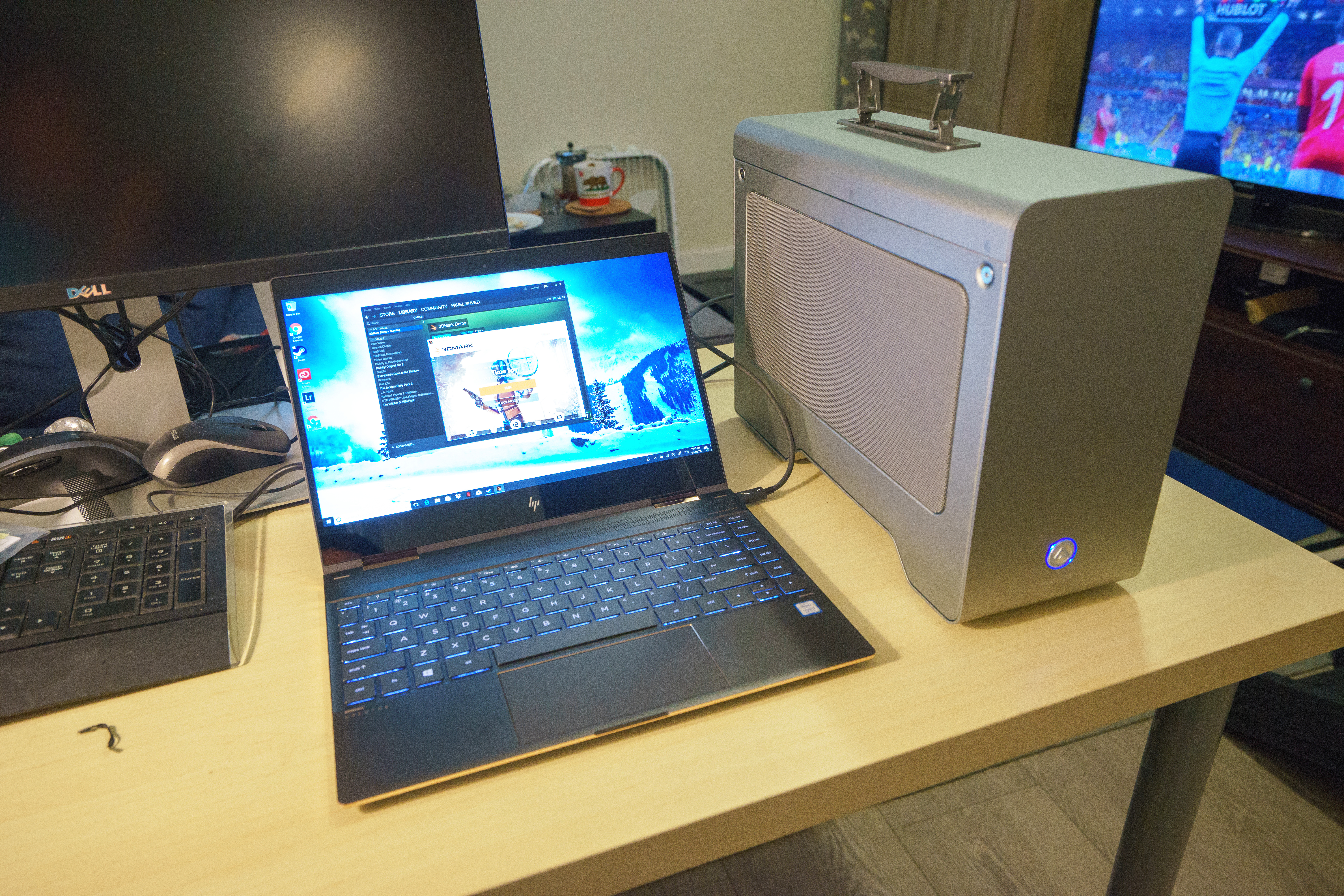
A Thunderbolt 3 external GPU setup that doesn’t weigh 7 pounds (3kg)? Is it even possible? Of course it is, but you’ll need to do some simple tinkering. This post describes how you can do it in a couple of hours if you’re so inclined. You too can loose 4lbs off your Thunderbolt 3 eGPU within a day!

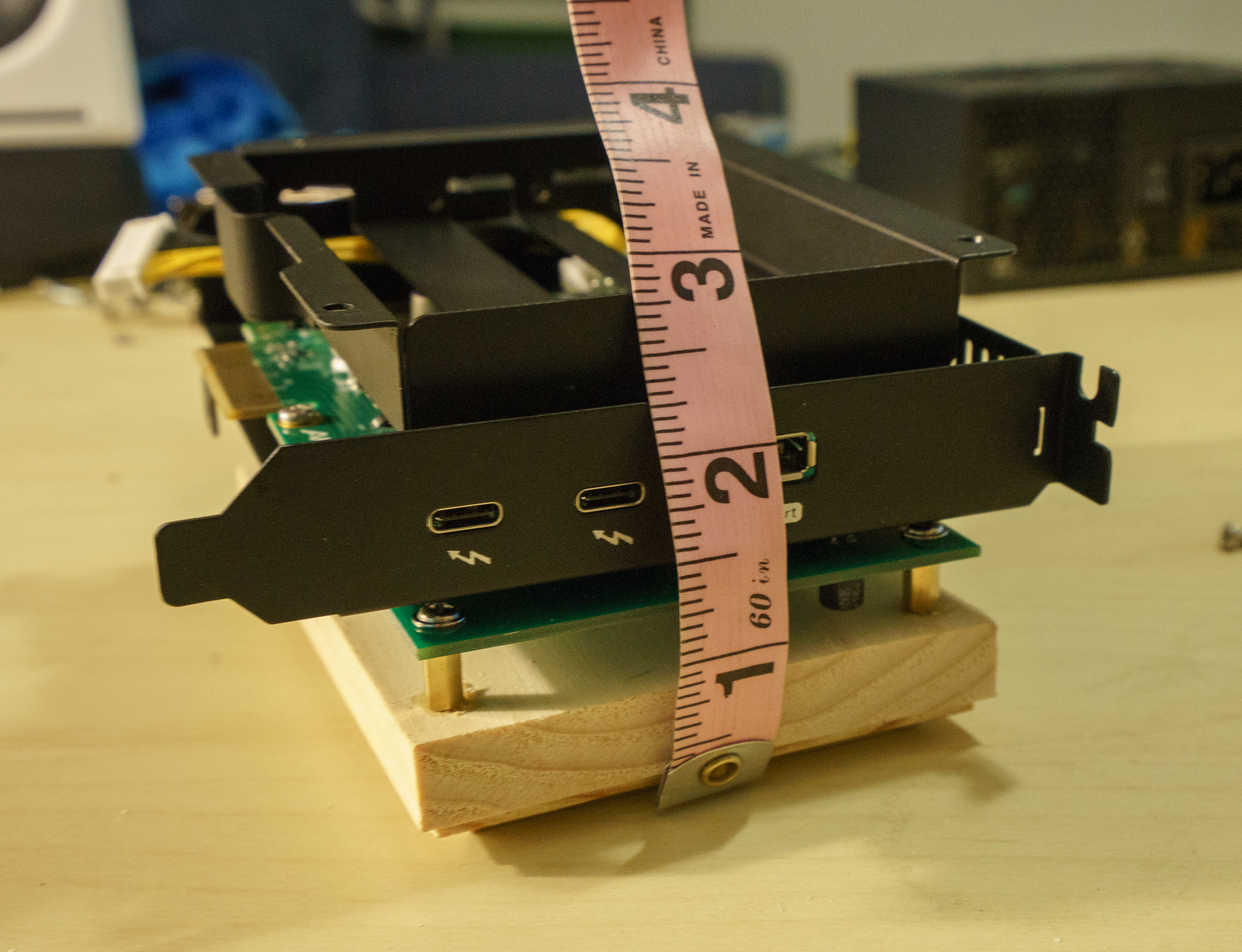
This is a Thunderbolt3-enabled DIY setup based on the Thunderbolt3-enabled components sourced from Akitio Node Pro (this and other Amazon links are affilliate). This is not the first of its kind. Here’s an example from Dec 2016 linked to me on reddit. And there are many other well-known DIY setups for pre-TB3 tech [1] [2]. My setup weighs 1.5kg including the power supply, and only 0.47kg without one, and it can fit larger video cards.

This setup does not aim to save money, but to achieve superior portability, utilizing Thunderbolt3’s plug-and-play capabilities as well as keeping it light and small. It cost about $400, but at least it doesn’t needs its separate suitcase now!

Shortly after assembling the setup, the Akitio Node’s power supply unit I’ve extracted went bust. I’ve initially replaced it with a regular desktop PSU since that’s what my local hardware store was carrying. However, I’ve since upgraded the setup to a more compact PSU, Corsair SF600. That way, the entire setup still weighs 1.3 kg.

If you want to skip my rambling about GPUs, laptops, portability, and the good old days of the greener grass, you may scroll straight to the assembly guide, and check out more pictures with the completed setup Otherwise, read on.

And if you own a business that produces the Thunderbolt 3 enclosures, could you please pretty please just make a retail solution that weighs 2 lbs, 75% of which would be the power supply? Please?

On 4k screens, portability, and priorities

Would you believe that an employed, experienced software engineer does not own a laptop? Neither did my friends whom I told I don’t own one. Boy did it make for some awkward job interview conversations. “Let’s code something on your laptop!” and I would respond, “Oh I don’t own one,” and get this suspicious “oh really” squint.

(Answer: I just don’t.)

I finally gave in when gearing up for a vacation in my hometown. I recalled all the times I wanted to use a laptop: mostly when writing blog posts on an airplane (like this one), researching bike routes when traveling, and editing photos I’ve just taken. Many of these tasks have been mostly, but not completely replaced by smart phones (Lightroom for phones and shooting RAWs from a phone camera dealing a pretty severe blow).

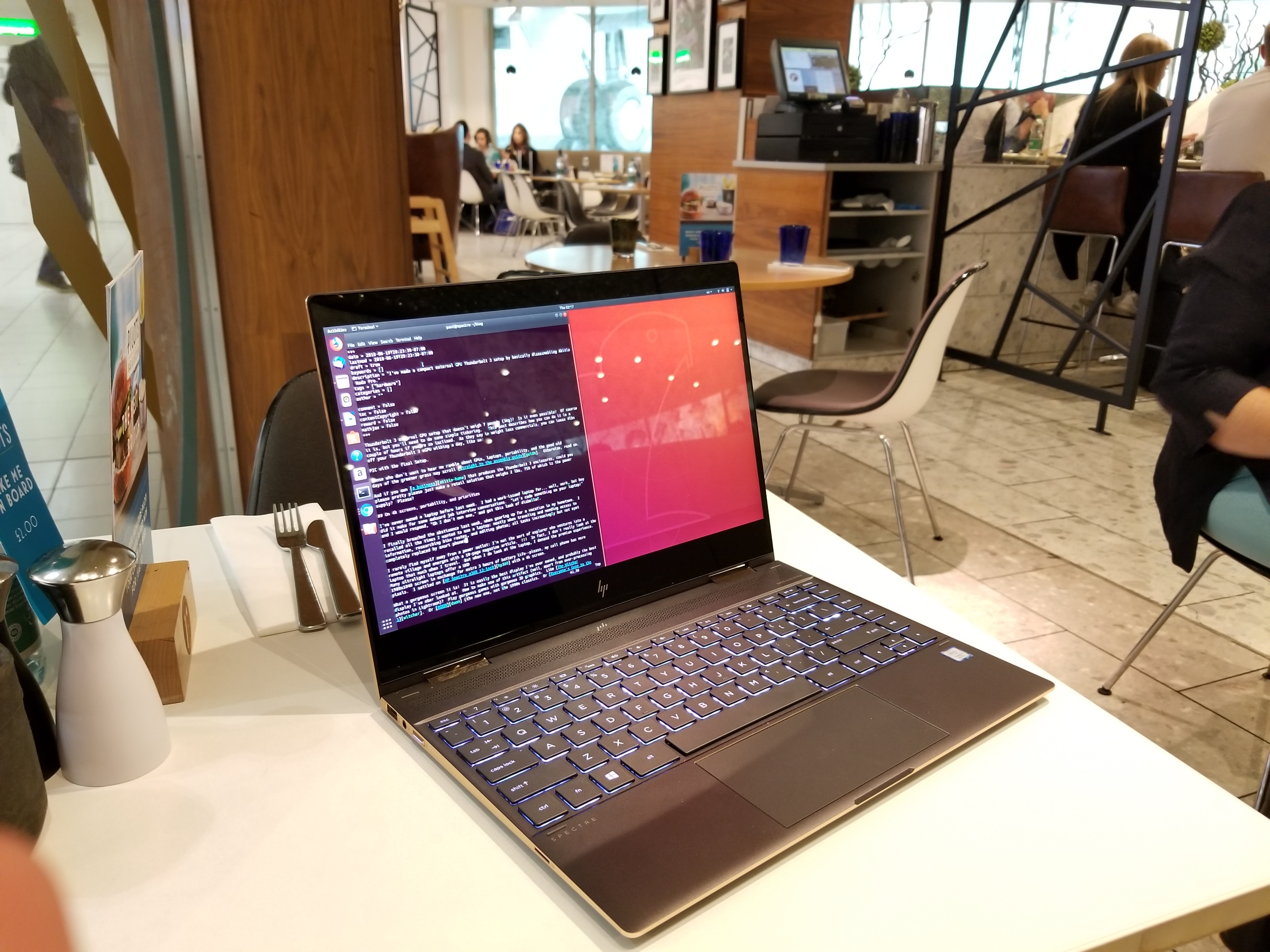
I rarely need a laptop when away from a power outlet: I’m not the sort of explorer who ventures into a remote village and emerges with a 10-page magazine article. In fact, I don’t really look at the laptop that much when I travel. But when I do look at the laptop, I demand the premium experience. Many ultralight laptops offer a UHD 1980x1040 screen in exchange for the extra 2-3 hours of battery life… Please, my cell phone has more pixels! I settled on HP Spectre x360 13-inch with a 4k screen.

What a gorgeous screen it is! It is easily the best display I’ve ever owned, and probably the best display I’ve eber looked at. How to make use of this artifact (well, apart from over-processing photos in Lightroom)? Play gorgeous games with gorgeous 3D graphics. Like The Witcher 3. Or DOOM (the new one, not the 1990s classics). Or Everyone’s Gone to the Rapture‘s serene landscapes.

The problem is, for a screen this gorgeous, the Spectre’s internal video card is simply… bad. The integrated Intel UHD 620 graphics card does not believe in speed. After rendering just 1 frame of the idyllic British countryside, the video card froze for 3 seconds, refusing to render another one frame until it’s done admiring the leaves, and the shades, and the reflection. It produces less than 1 FPS at best, and its 3DMark score of 313 solidly puts it at the worst 1% of computers to attempt the test.

The test doesn’t favor the brave–who would attempt to 3dmark an integrated ultralight laptop video card?–but it does show you how bad the result is. How can we improve?

When my desktop PC’s GeForce 660 MX saw the first frame of DOOM, it was in simiar awe, confused, confronted with a task more demanding it ever had before. After struggling a bit and rendering maybe three frames, the video card decided to retire, pack its things and move to Florida, while I replaced it with the state-of-the-art-but-not-too-crazy GeForce GTX 1070. DOOM instantly became fast and fun. So the question is now obvious.

How can I connect my allmighty GeForce GTX 1070 to the Laptop?

DIY eGPUs (before Thunderbolt 3)

Turns out, tinkerers have been connecting external GPUs to laptops since forever. With time, GPUs required more and more power and space, while the possible and hence demanded laptop size shrank. The GPU power consumption trend has finally been reversed, but the laptops are going to get lighter still.

A laptop is just a PC stuffed into a small plastic case, so connecting a GPU would be just like connecting it to the desktop. Laptop manufacturers would leave a “PCI extension slot” either featured as a supported connector or at least available inside the case for the bravest to solder. There is a lot of external GPU (eGPU) do-it-yourself DIY [1] [2], [3], and out-of-the-box solutions available.

But then, Intel developed a further extension of USB-C called Thunderbolt 3. The previous USB interface generations were also named “Thunderbolt”, just the lightning was meek and the thunder unnoticed).

eGPU after Thunderbolt 3

Thunderbolt 3 is no magic. It’s simply a standard to produce USB chips with higher wattage and throughoput… so high and fast that it allows you to connect, say, displays or even graphic cards over USB. It “merely” quadruples the throughput of the USB 3 standard, and now you can do plug-and-play for your video card, eh? You would just buy a thing to plug your video card into, and connect that thing into USB. Easy!

So all I need is to buy that “thing”. Easy! There’s a plenty of Thunderbolt 3 “things”, here, take a look:

Notice something? That’s right, they all are freaking gigantic and weigh 3-4 times more than the ultralight laptop itself. Here, I bought one, and it’s a size of an actual desktop computer I own!

The manufacturers are telling: “want Thunderbolt 3? Buy a 3 kg case!” Look Akitio Node Pro has a freaking handle! A handle!

It didn’t use to be this way. Before Thunderbolt 3 enabled plug-and-play, hackers still found ways to attach an eGPU as shown above. These solutions are tiny and they cost pennies! How do we get something similar with Thunderbolt 3?

Some speculate Intel just takes a pretty big cut in the licensing fees for every Thunderbolt 3 device produced. Since they say it on the internet, it must be true. (See also here, scroll to the middle.) This explains the $200+ price. But that does not explain the 7 lbs of scrap.

It’s time to take the matter into my own hands.

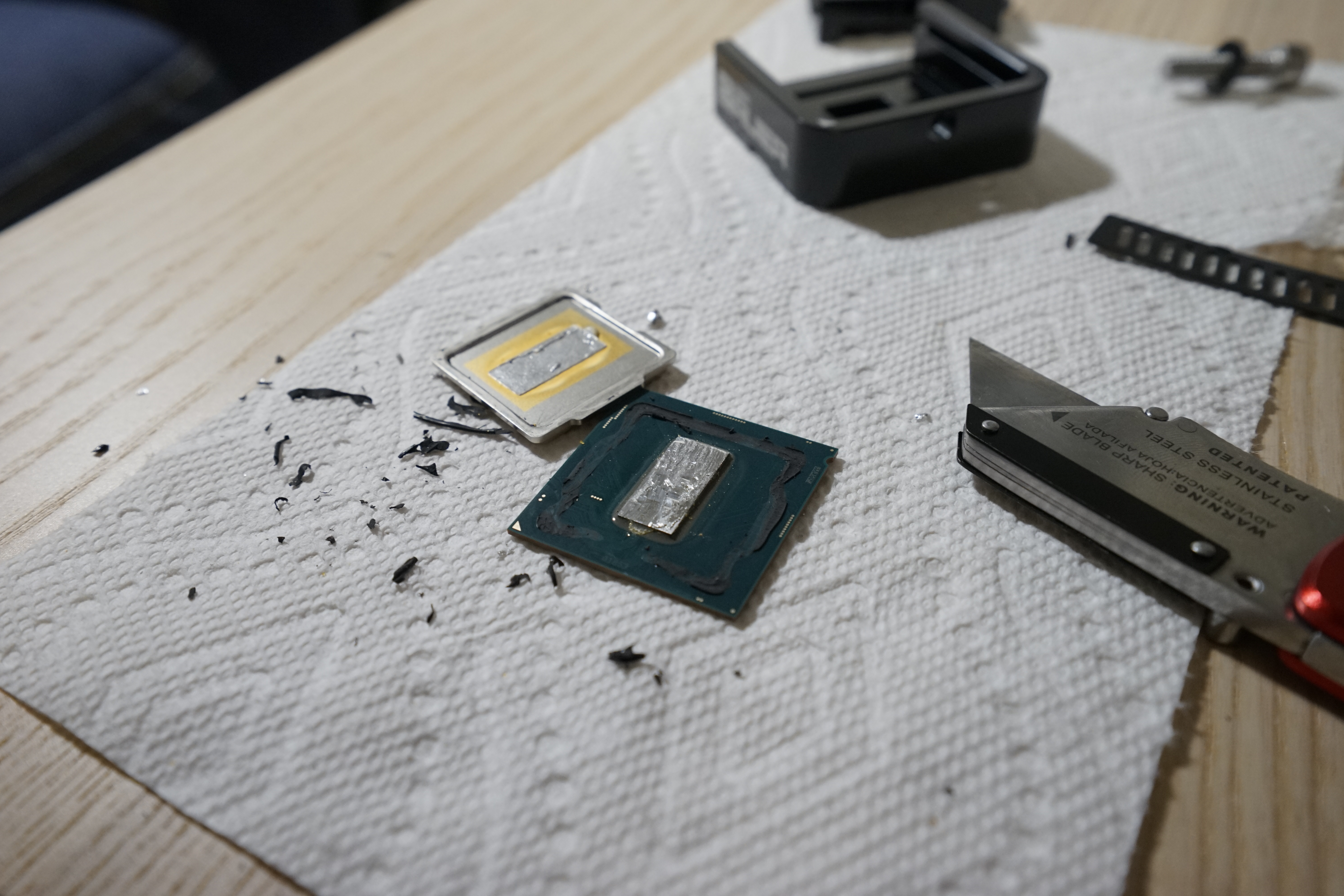
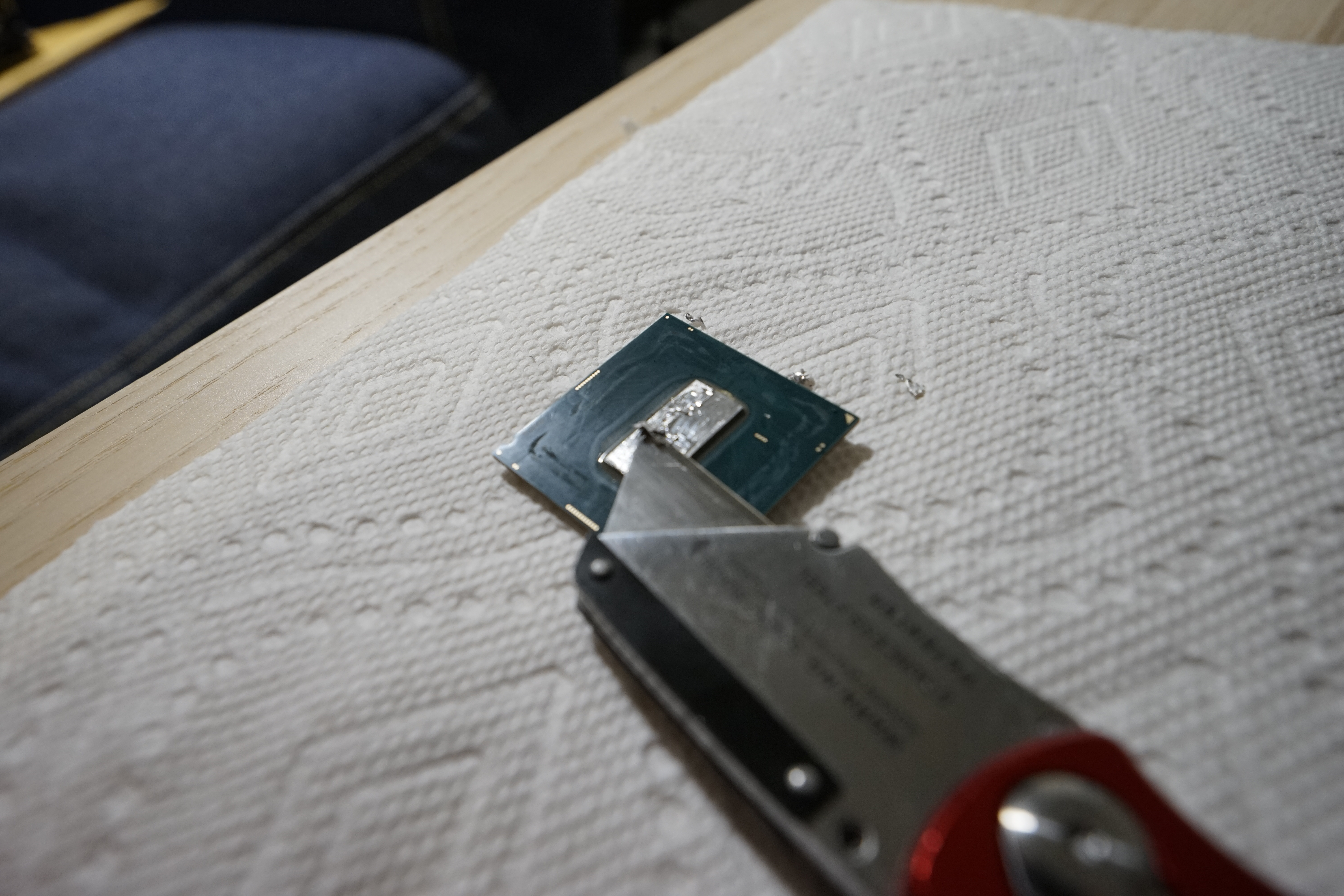
“When There’s Nothing Left to Take Away”

…perfection is finally attained not when there is no longer anything to add, but when there is no longer anything to take away. Quote: “Terre des Hommes” via wikiquote. – Antoine de Saint Exupéry

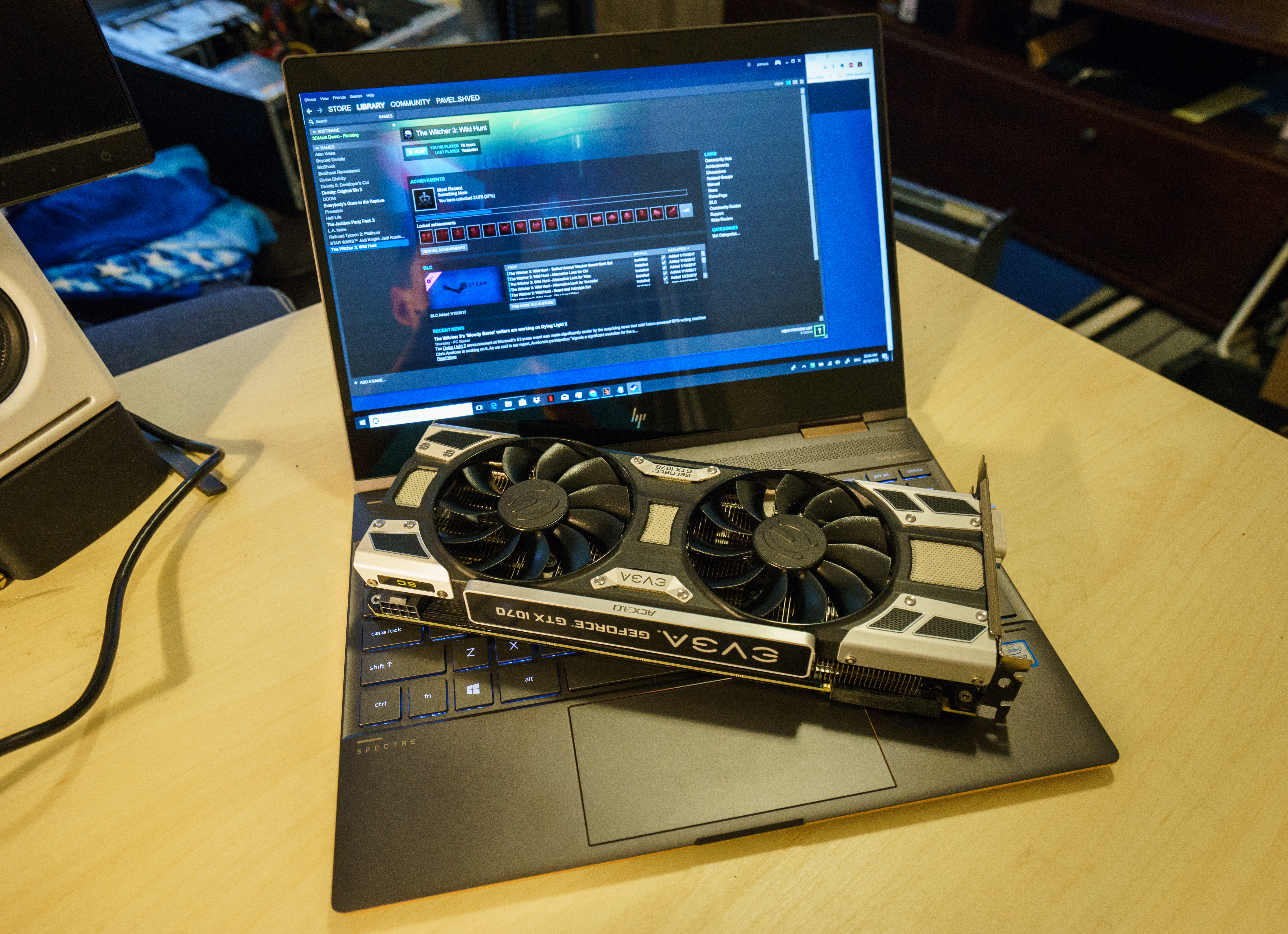
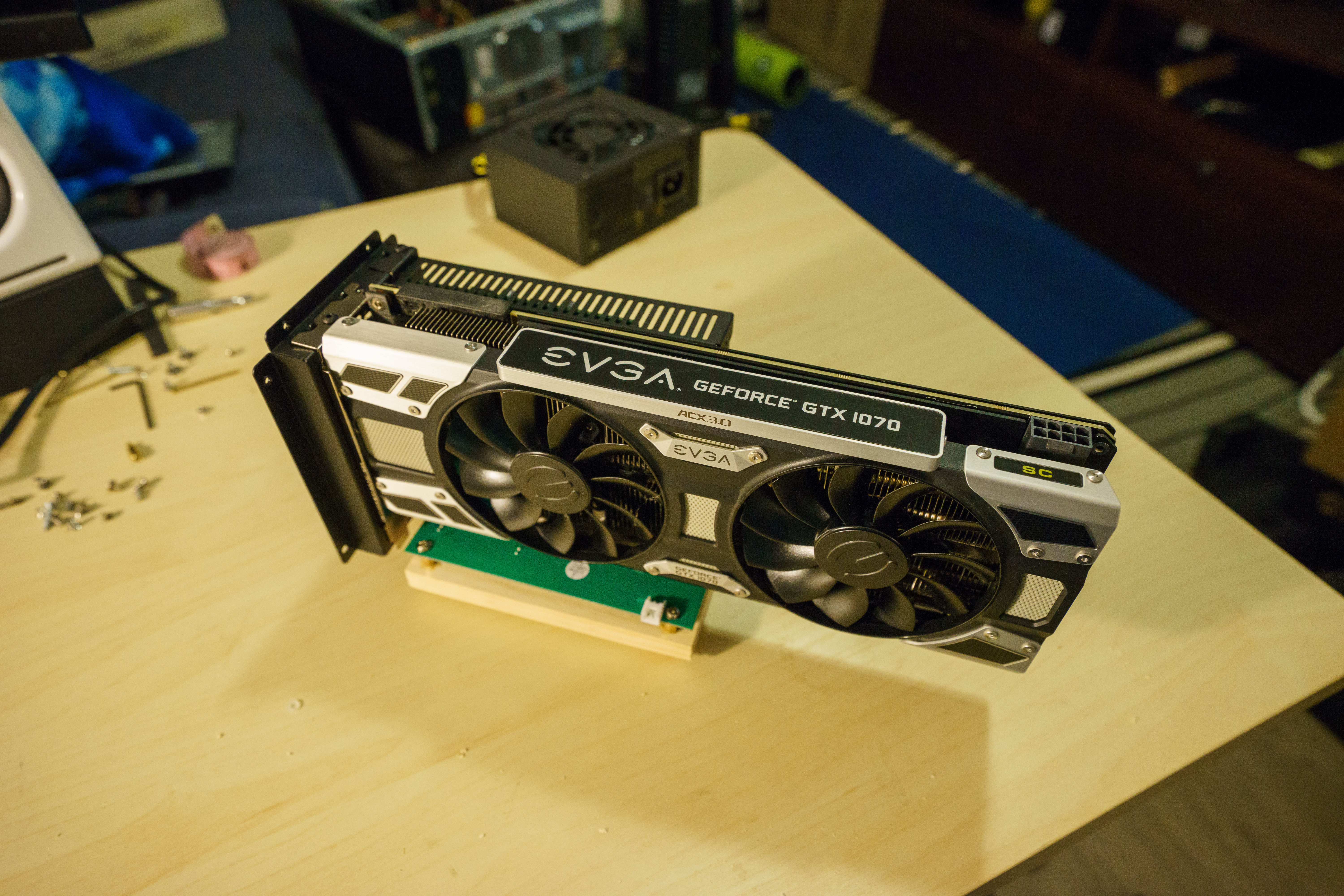
So we’re going to turn this

into this

The procedure consists of two steps: disassembling the original box, and mounting of the enclosure onto a chunk of wood. Before we start, please understand the risks of this procedure, and accept the full responsibiltiy for the results.

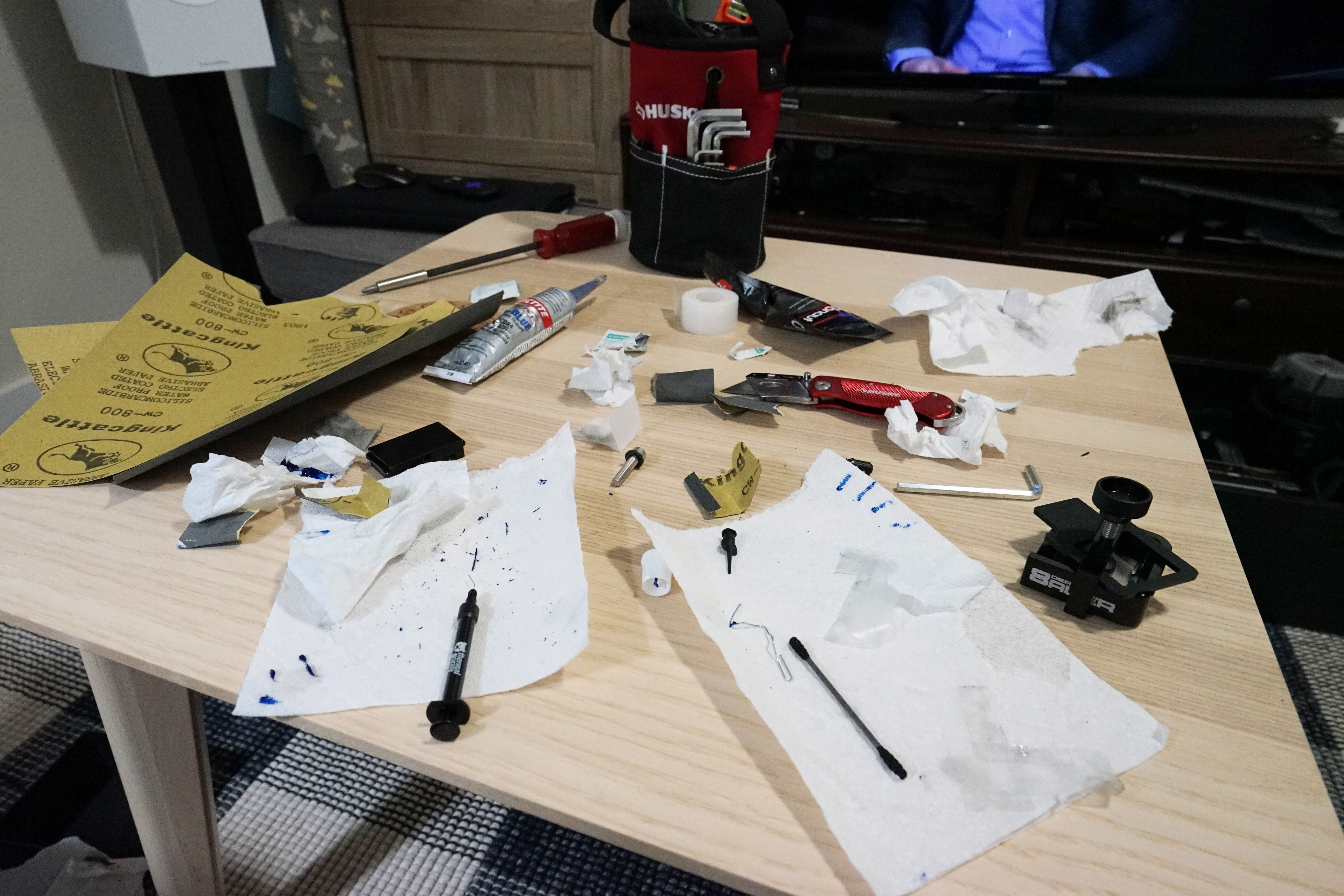
We’ll need the following ingridients:

• Akitio Node Pro (to source the TB3 extension cards) (amazon);
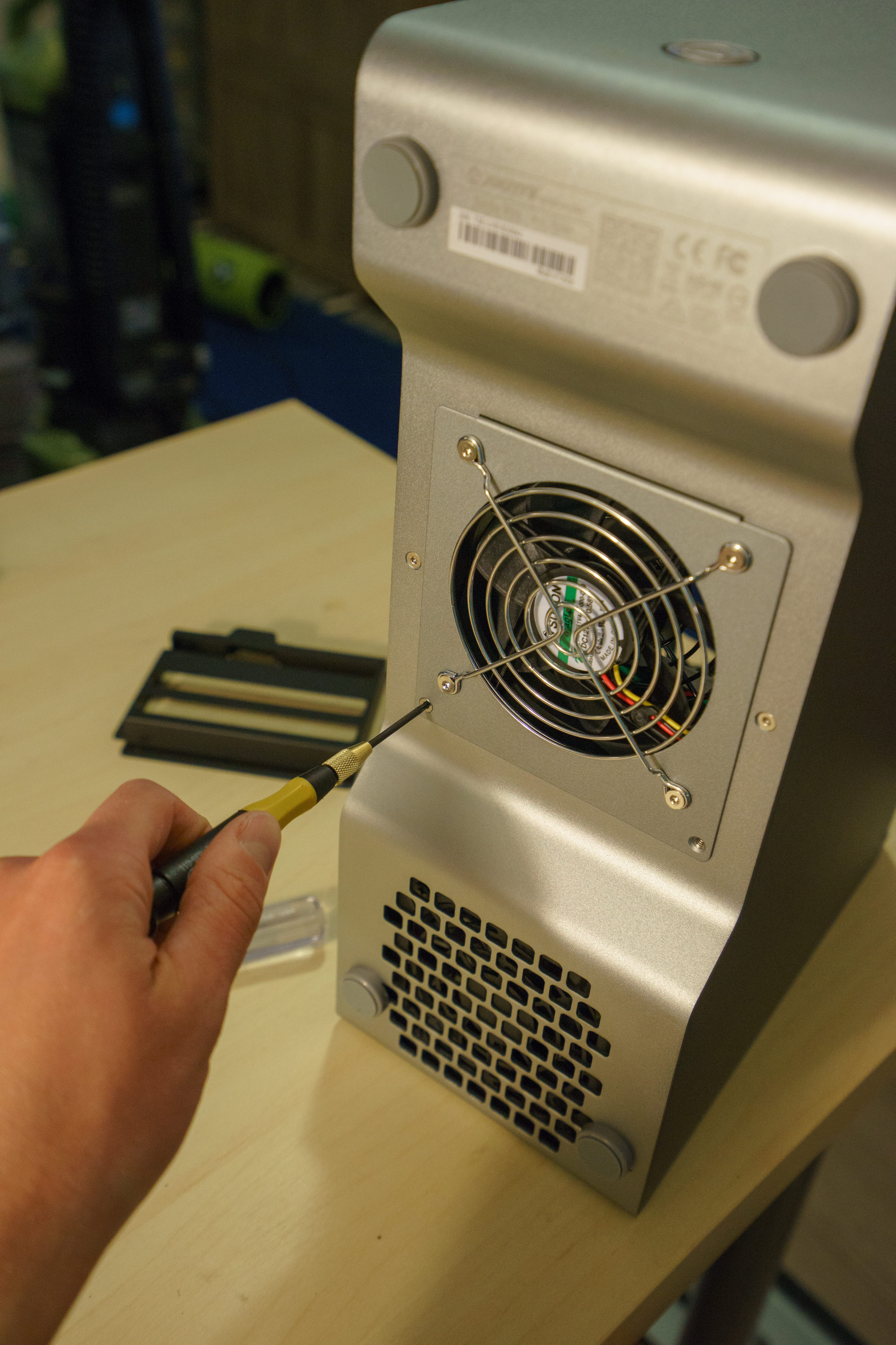
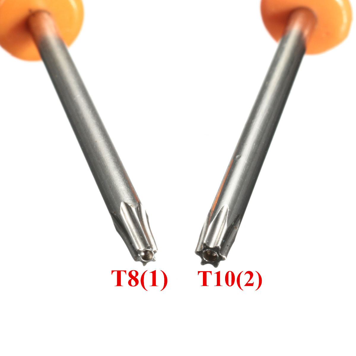
• T10 and T8 screwdrivers (to disassemble the case) (see the pic, and sample product);
• Set of M3 standoffs (at least half an inch tall); we’ll recycle the matching screws from the original assembly (amazon);
• Chunk of wood at least 3x5 inches (to mount the assembly onto) (amazon);
• Drill or some other way to make deep holes in the said wood;
• Super Glue (or some other glue to stick metal to wood)

A note on choosing the enclosure

The enclosure used here was Akitio Node Pro. I mostly chose it for these reasons:

1. a compact 500W power supply. I found the reports of its noisiness unwarranted, but I was a bit unlucky with it.
2. existing evidence it’s ieasy to take apart
3. a proven record of its compatibility with GTX 1070.
4. powerful enough to also charge the laptop (unlike, say, the non-“Pro” Akitio Node)! I can confirm it does. You should shoot for 450-500W+ for that: the laptop charger would draw 100W, and you can look it up in the reviews.
5. … and last but not least it actually scored well in the reviews (see also the comparison).

Taking the case apart

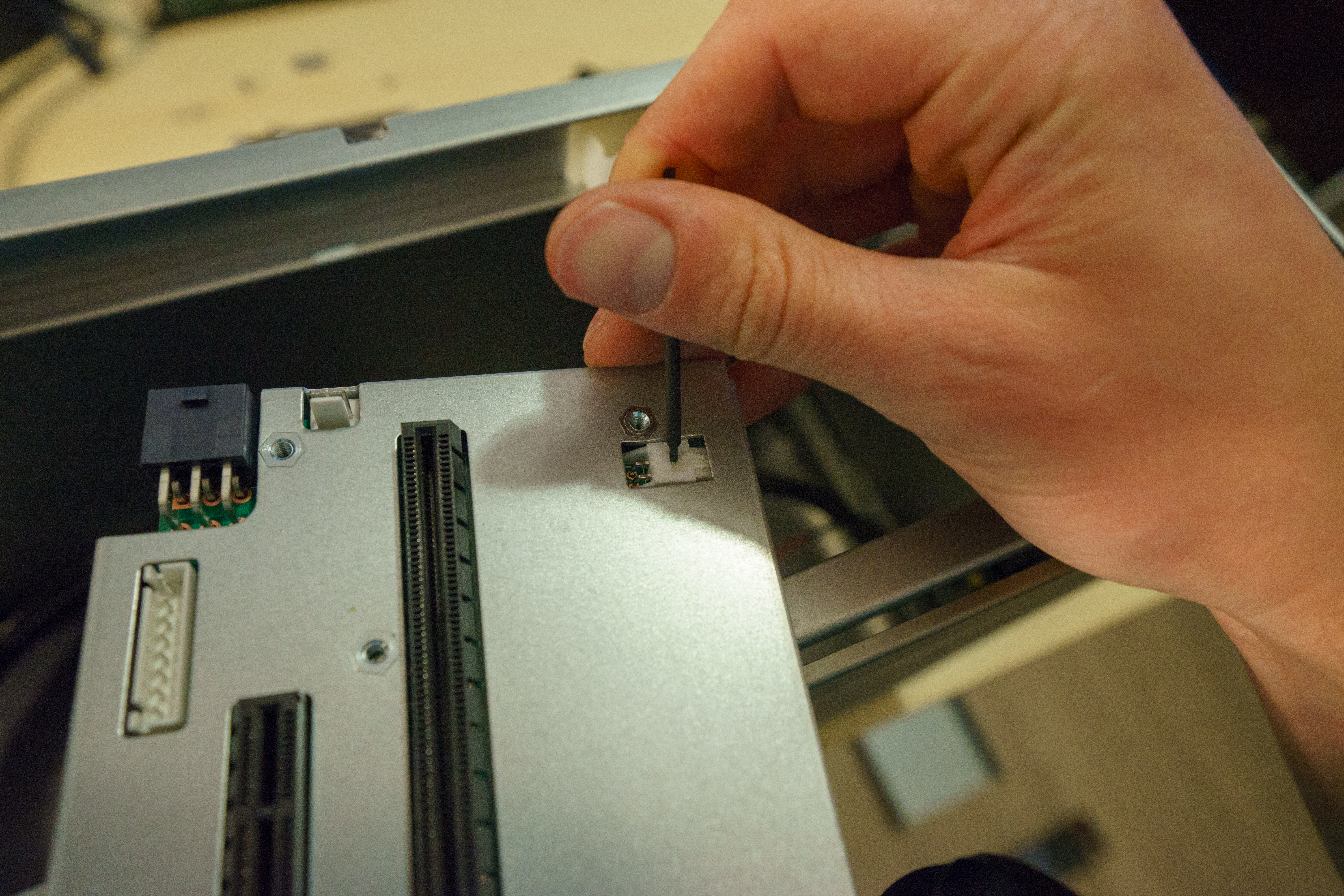
It was somewhat straightforward to disassemble the box. I needed T8 and T10 screws as well as the expected Phillips screw. I got T8 and T10 from ACE Hardware brick-and-mortar stores. If you’re curious, hex screwdrivers and flat screwdrivers only got me so far, until I faces a Boss Screw, a T10 right next to a board. That’s when I gave up and went to the hardware store:

Basically, just unscrew every bolt you can see, remove the part if you can; then find more screws and repeat.

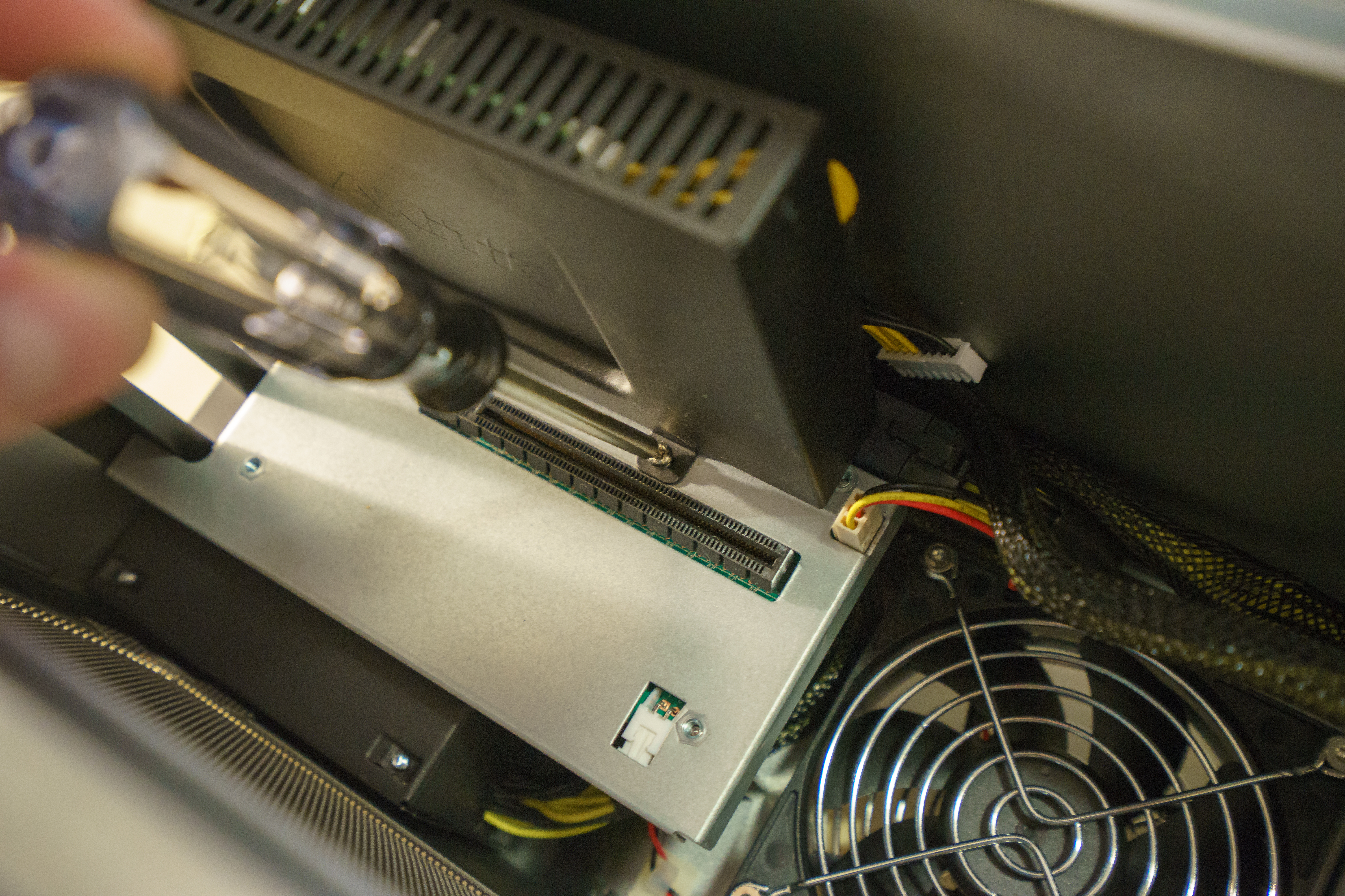
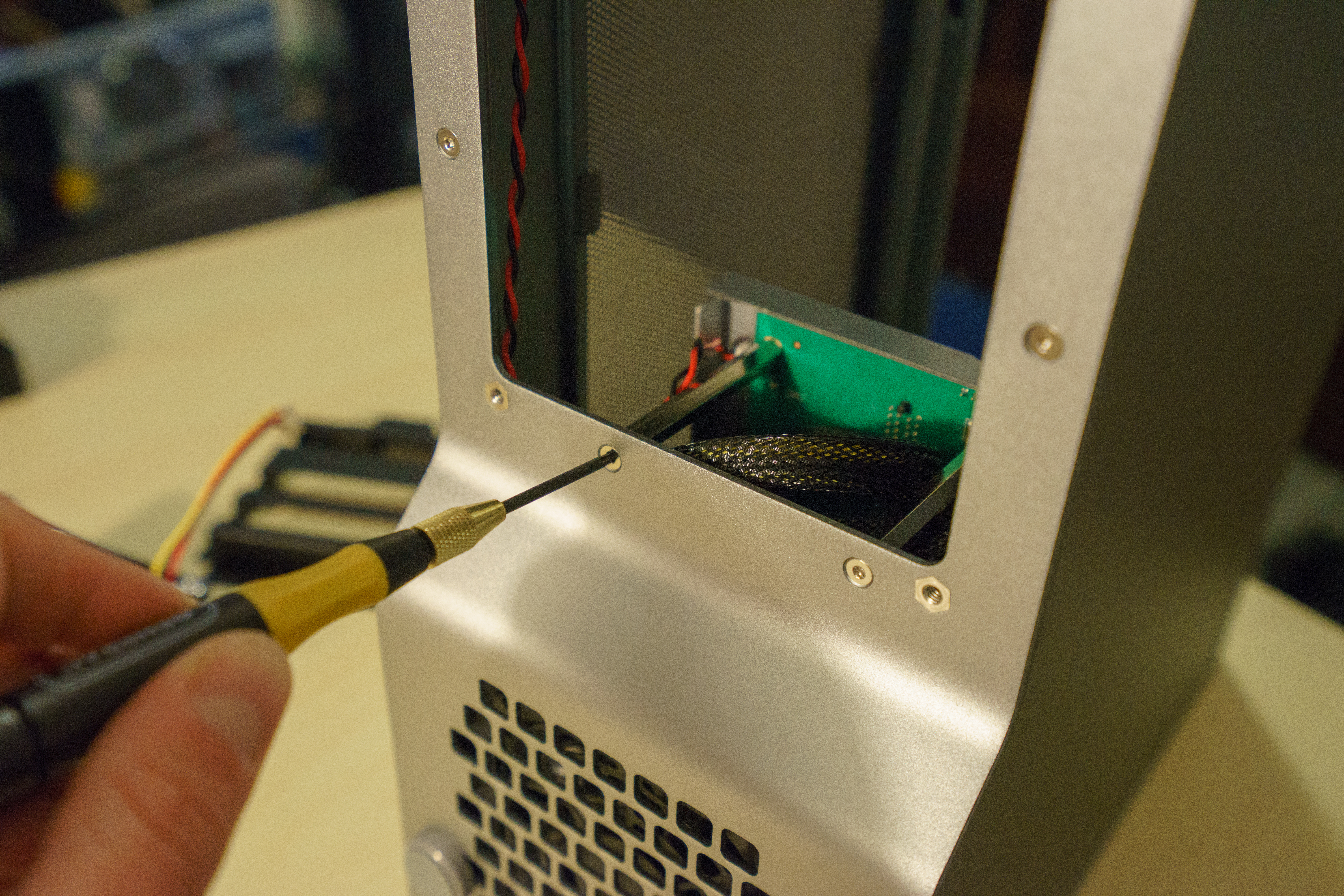
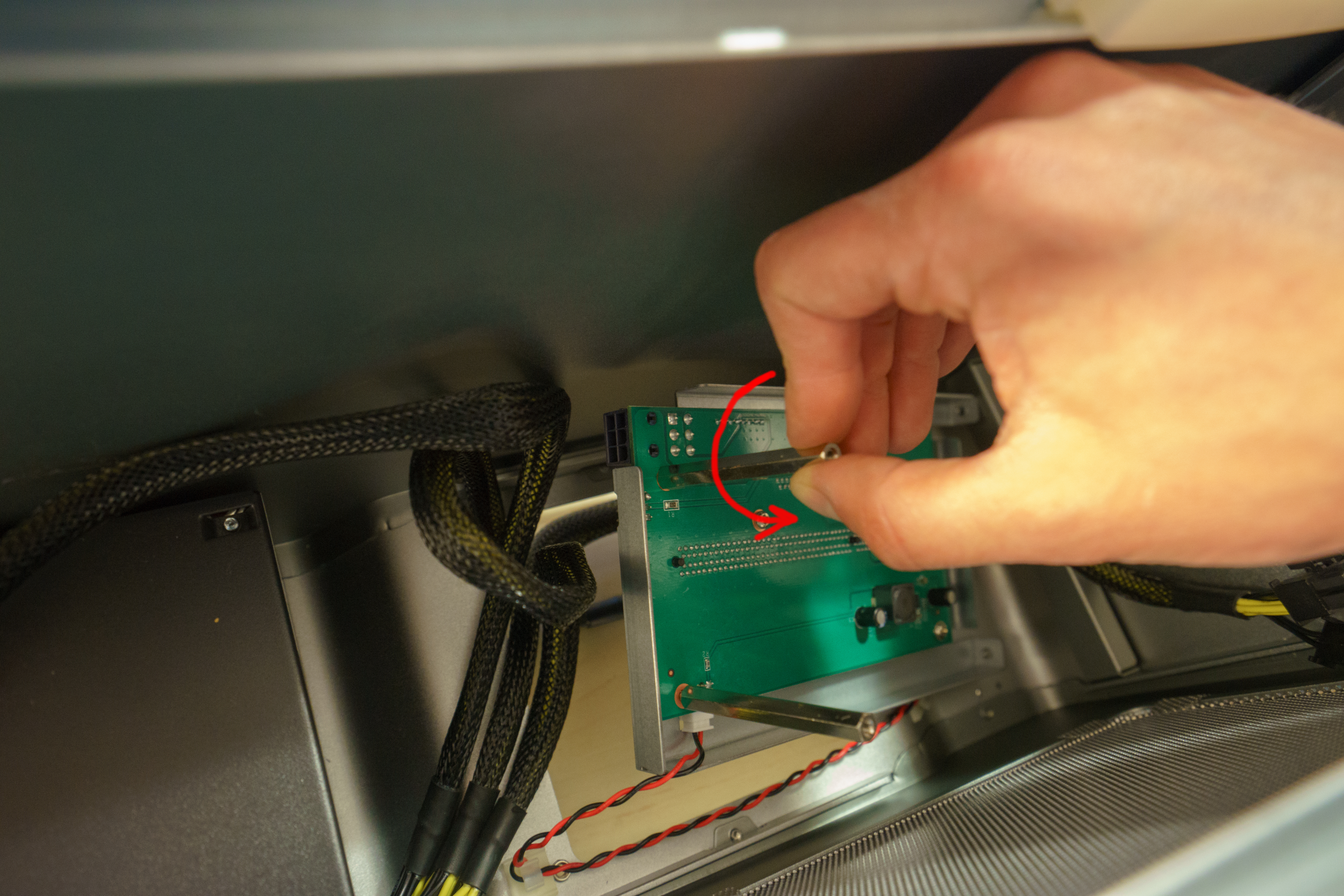
This bit is tricky: you need to unplug this wire; I couldn’t find more ways to unscrew anything else, so I just extracted this using a thin Allen key.

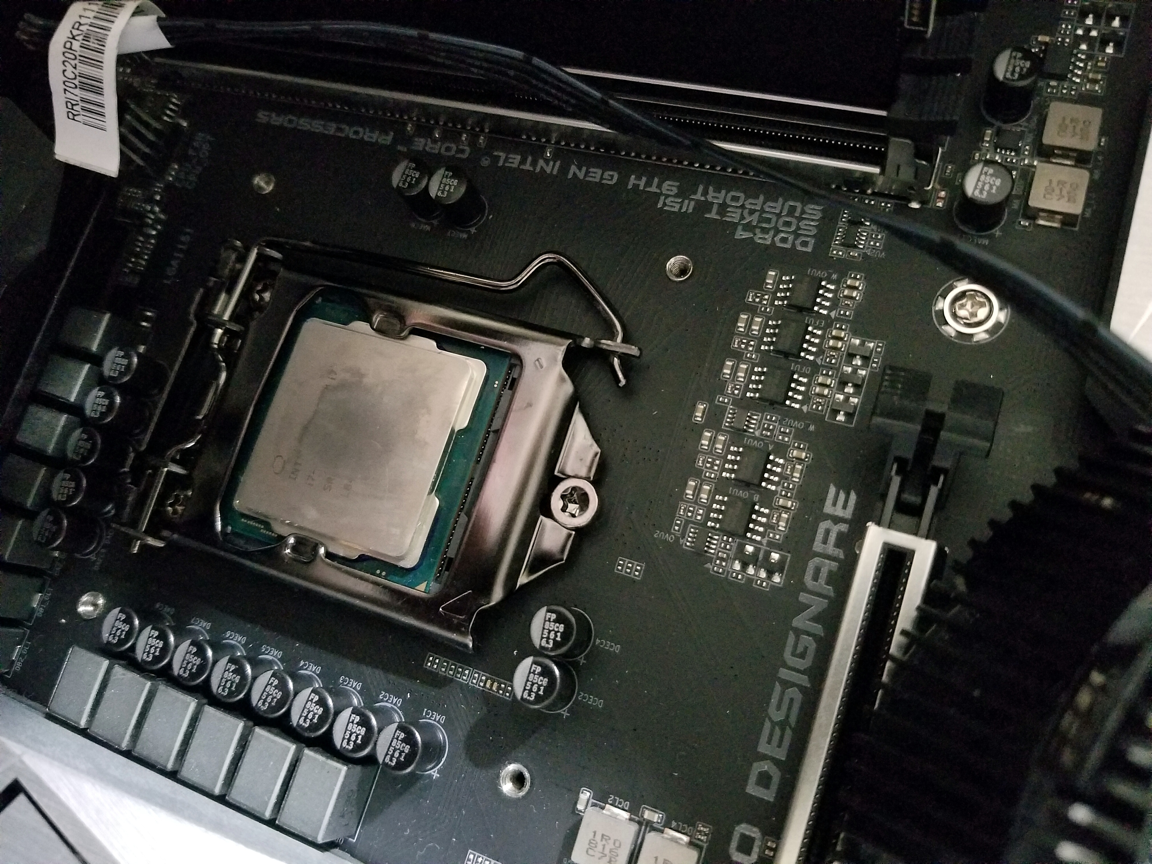
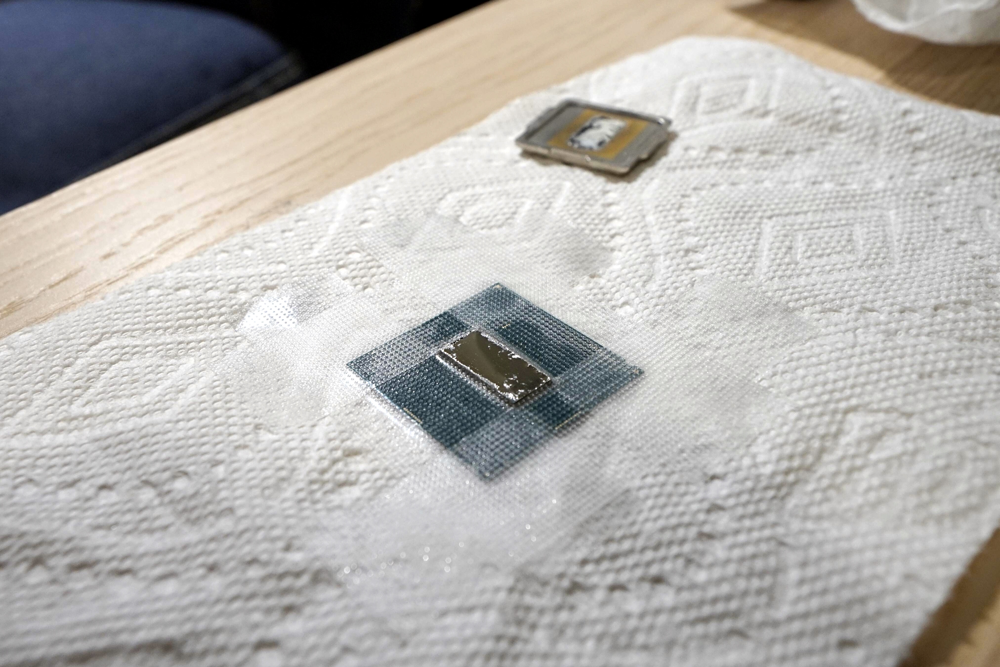
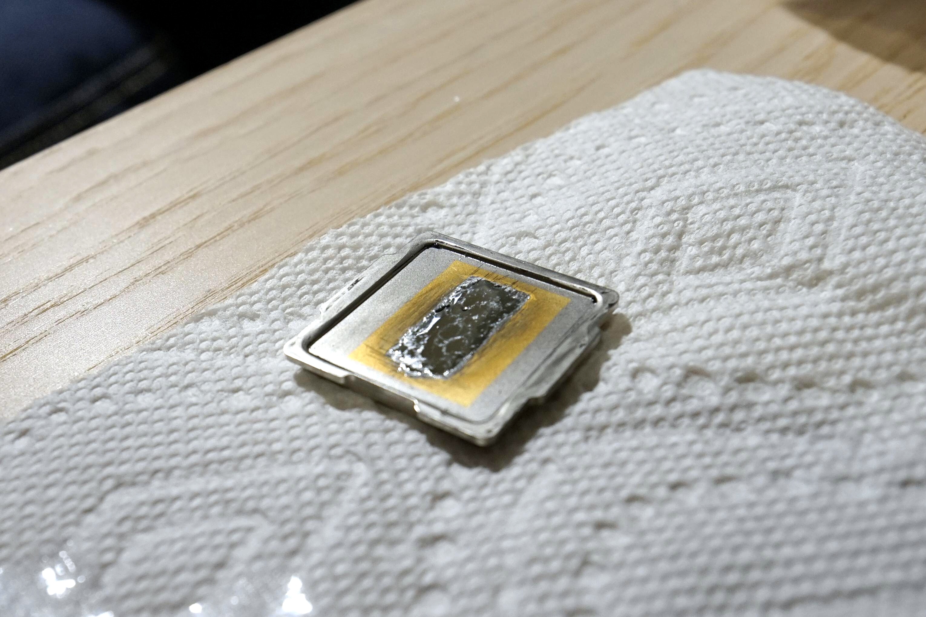
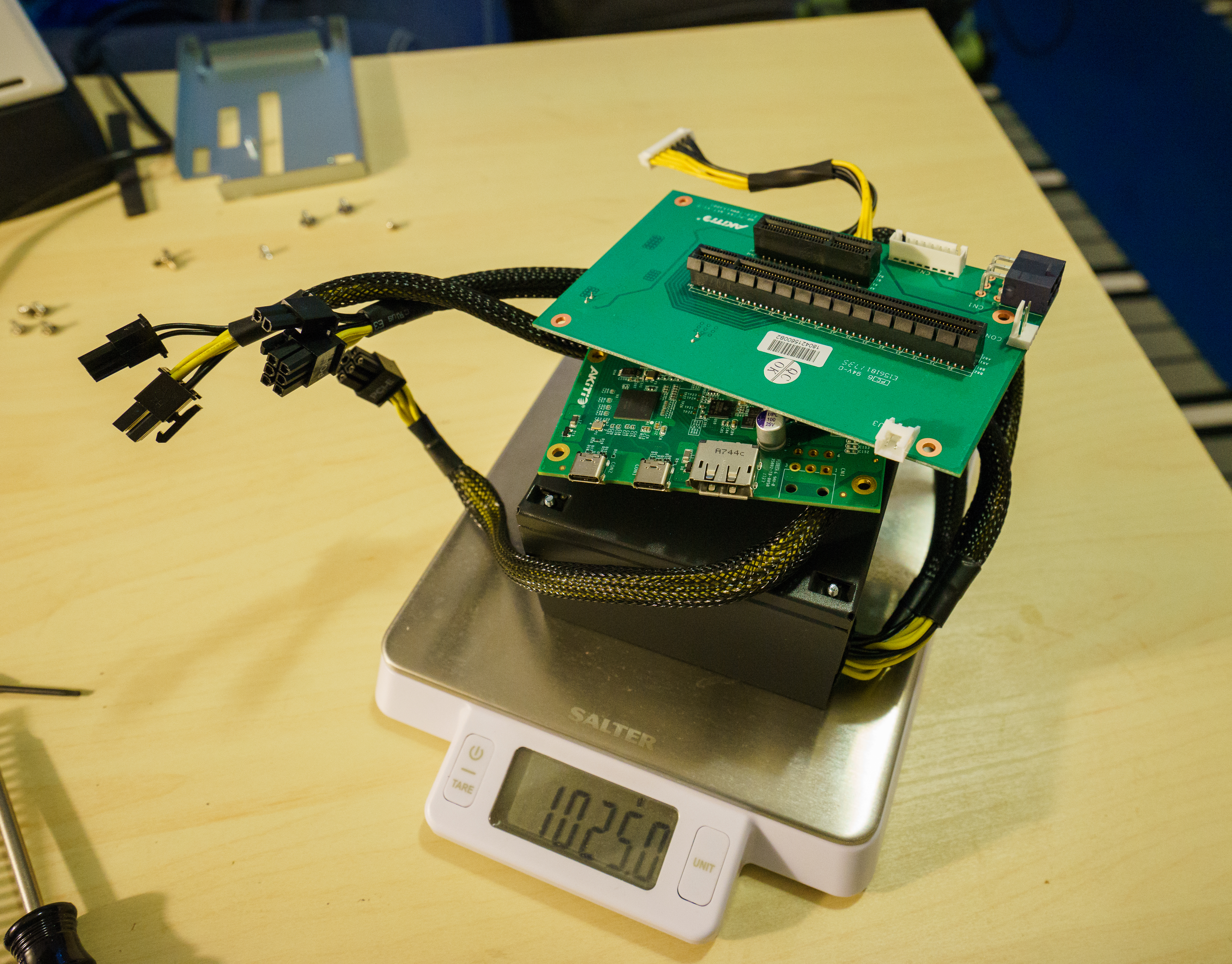
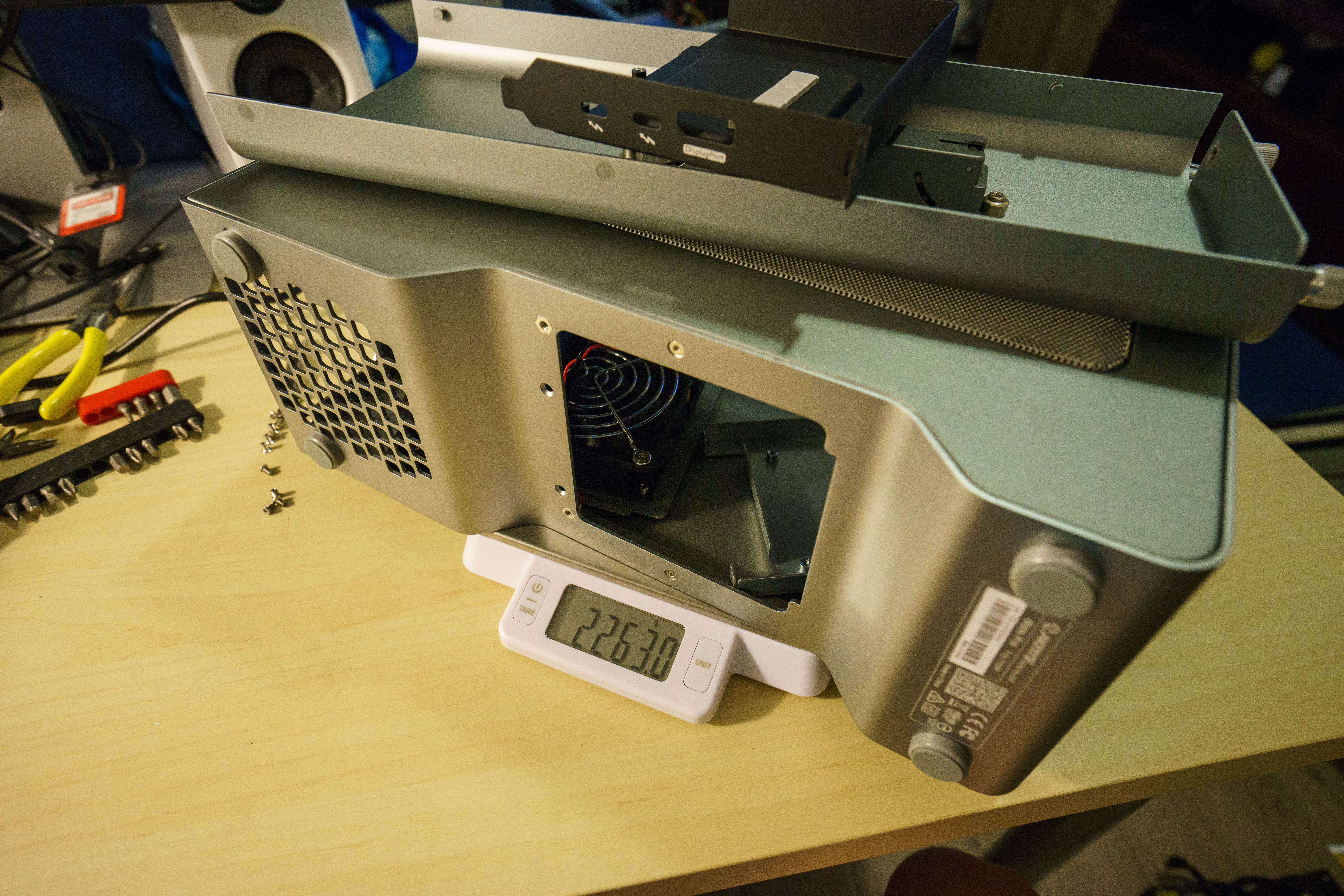
What we need is these three parts: two boards (one with the PCI slots and the other with the USB ports), and the power supply. Look, they weigh only 1kg, as opposed to other, non-essential parts that weigh 2.3kg.

Putting it back together (without the scrap)

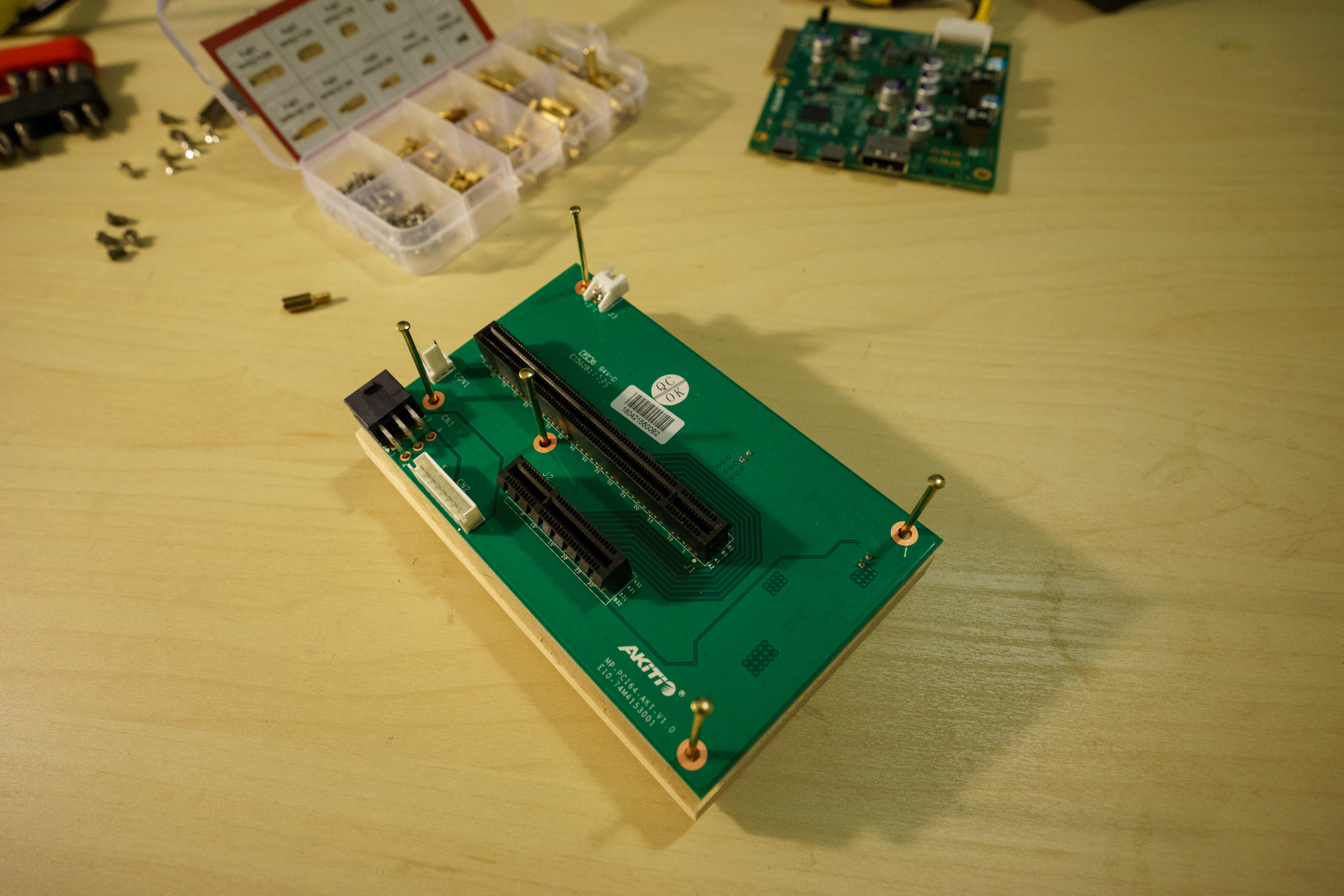
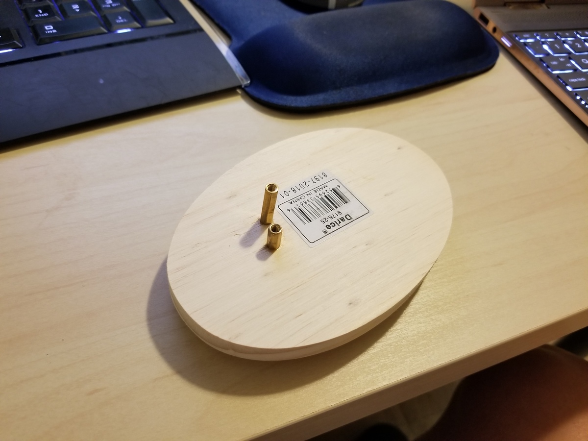
The bottom board, once dismounted, reveals that it can’t stand on its own and needs to be mounted on at least 1cm standoffs. I decided to mount them onto a wooden board that needs to be at least 3x5. This board set worked, albeit it only had 1 out of 5 boards that was rectangular (it fits pretty snug so you only have one chance).

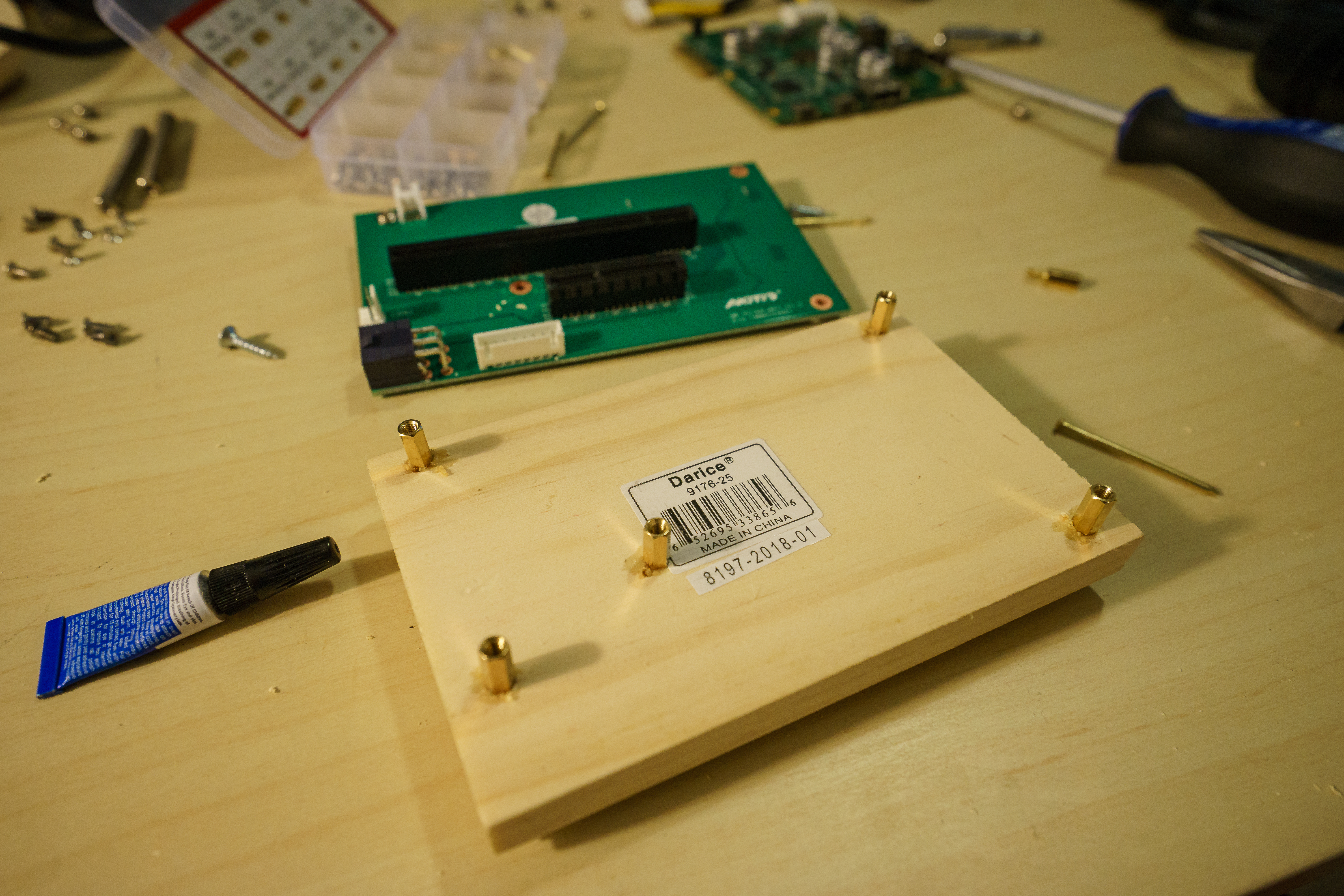
Wait, how did I know where to put those, and how did I secure them? Simple: I drilled the wood and glued the standoffs. I first tried to mark the spots to drill by putting nails through the mount holes like so:

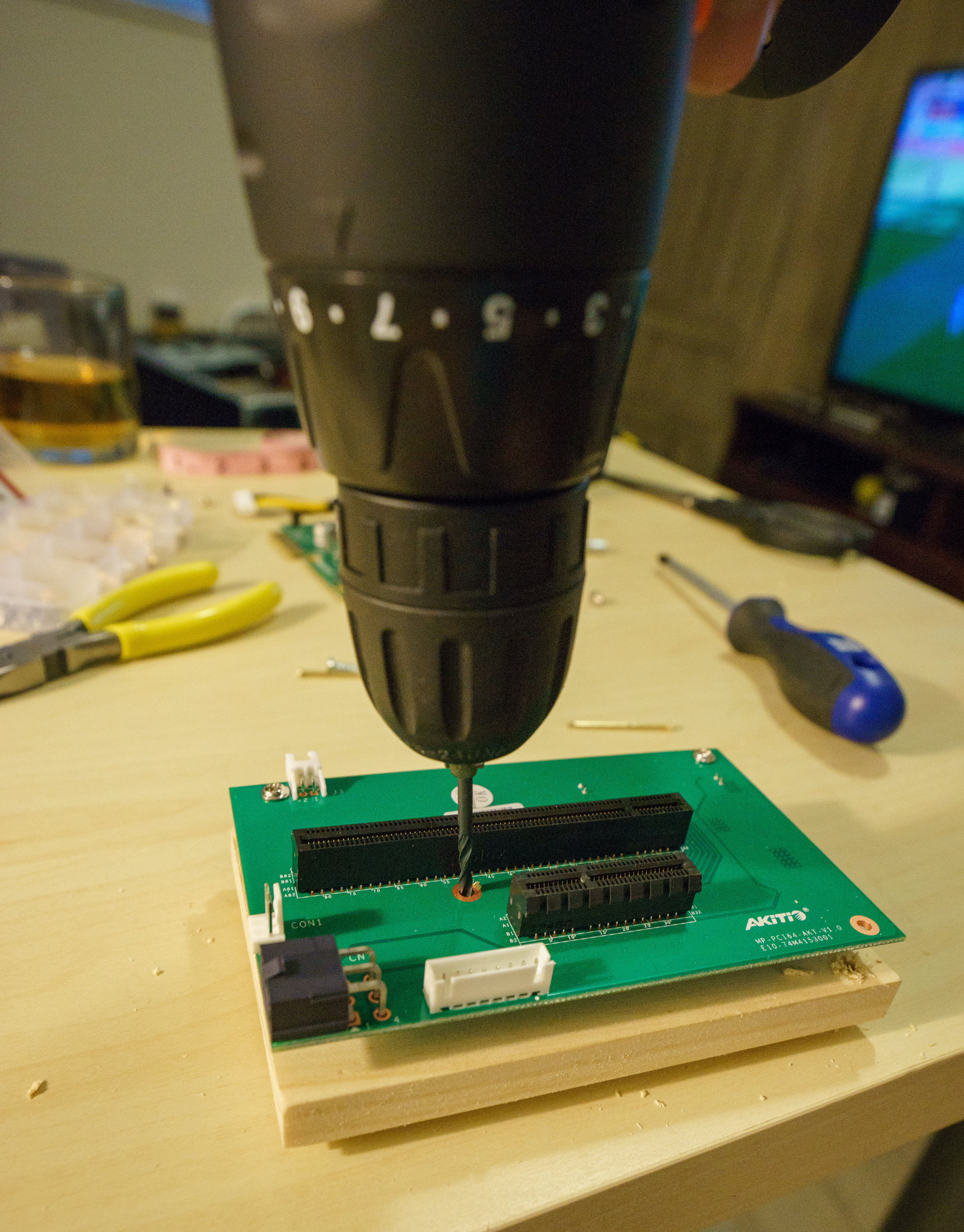
This did not work! I wasn’t able to put the nails in straight enough, and missed the correct spot for a millimeter or so. I fixed it by tilting one of the standoffs a bit, but I did resort to a different method of marking the holes: drilling right through the board!

This looked sketchy but it worked better than trying to hammer nails vertically.

I used super glue to secure the standoffs to the wood. As added security, I put a bit of saw dust back into the holes for a tighter grip. (Ask Alex for the right way. Some mention epoxy glue but then my dad said its unsuitable for gluing wood to metal, so I didn’t research this question further (and I surely didn’t have it and I didn’t want to go to the hardware store again).

I practiced to mount standoffs onto a different board first, and I highly recommend you do this too. I only had one board at the time, so I couldn’t screw it up, but if you just get more boards, it’d be easier.

Finishing touches and results

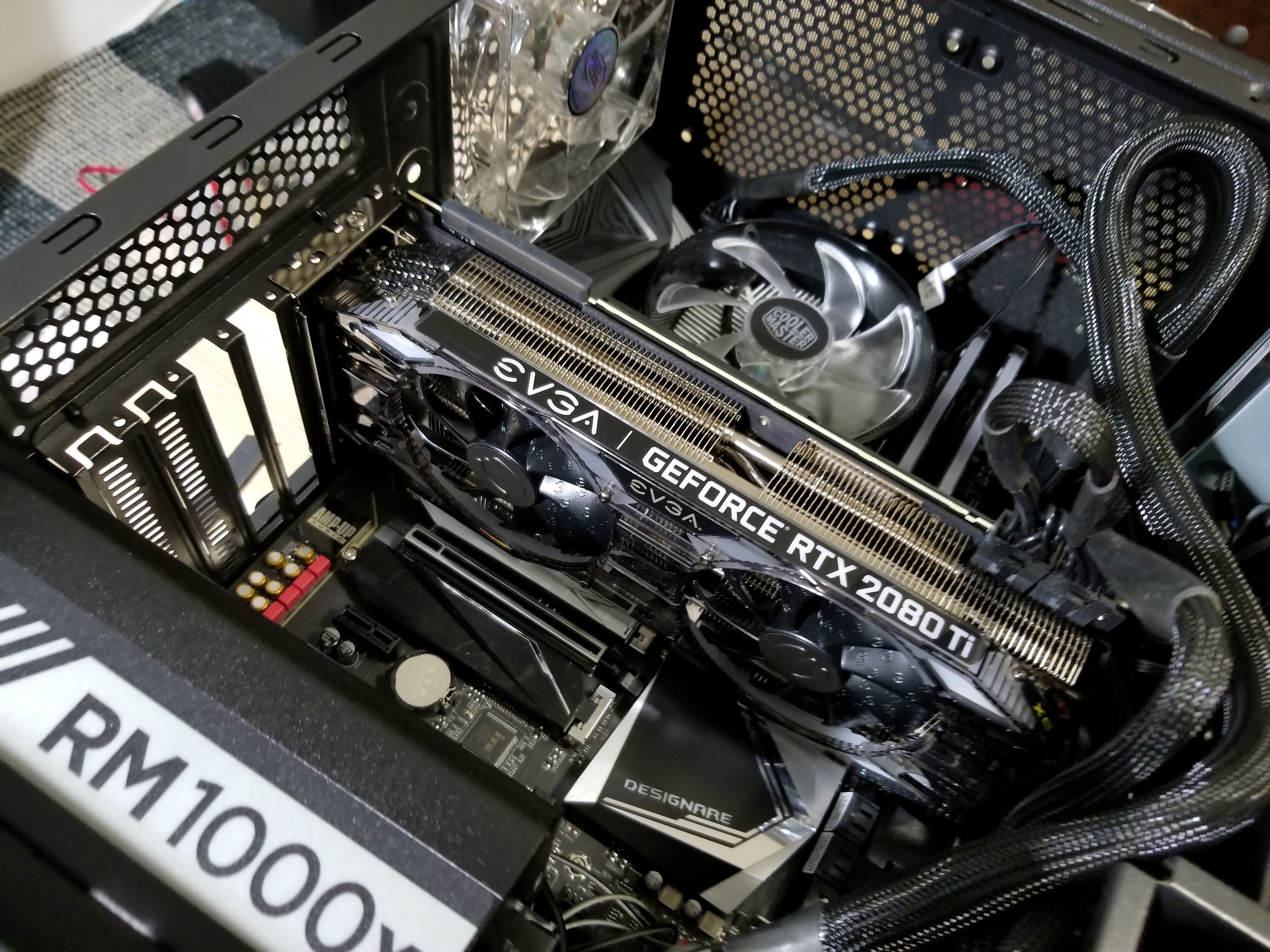
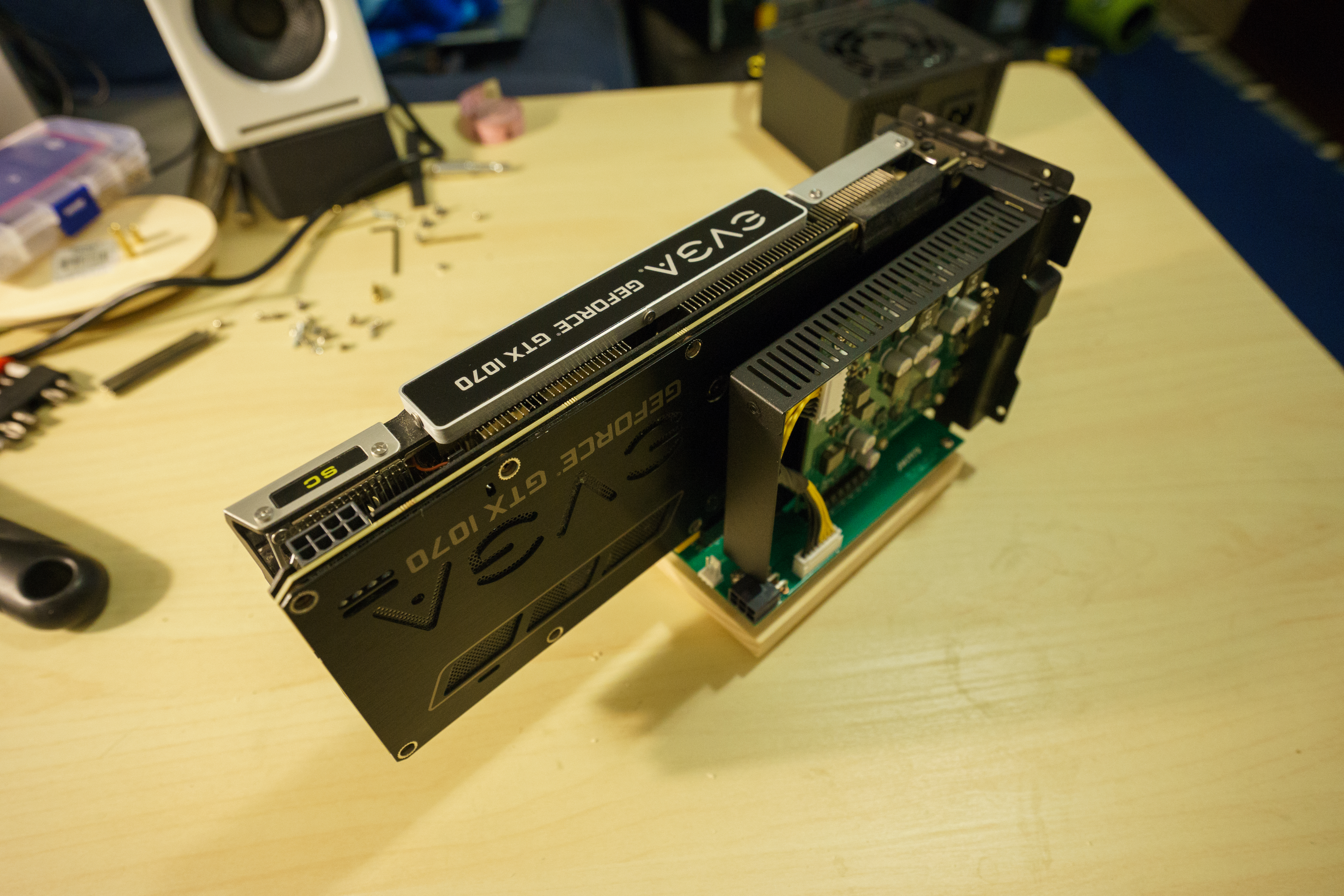
After I plugged the cards, the setup seemed a bit unstable. After all, that is a heavy double-slot monster of a GPU. So I added back one of the assembly pieces previously discarded and secured it back with a screw I found. However, I also later lost that screw while on the road, and ran this for hours without the extra piece, and it worked well, and didn’t fall over (duh).

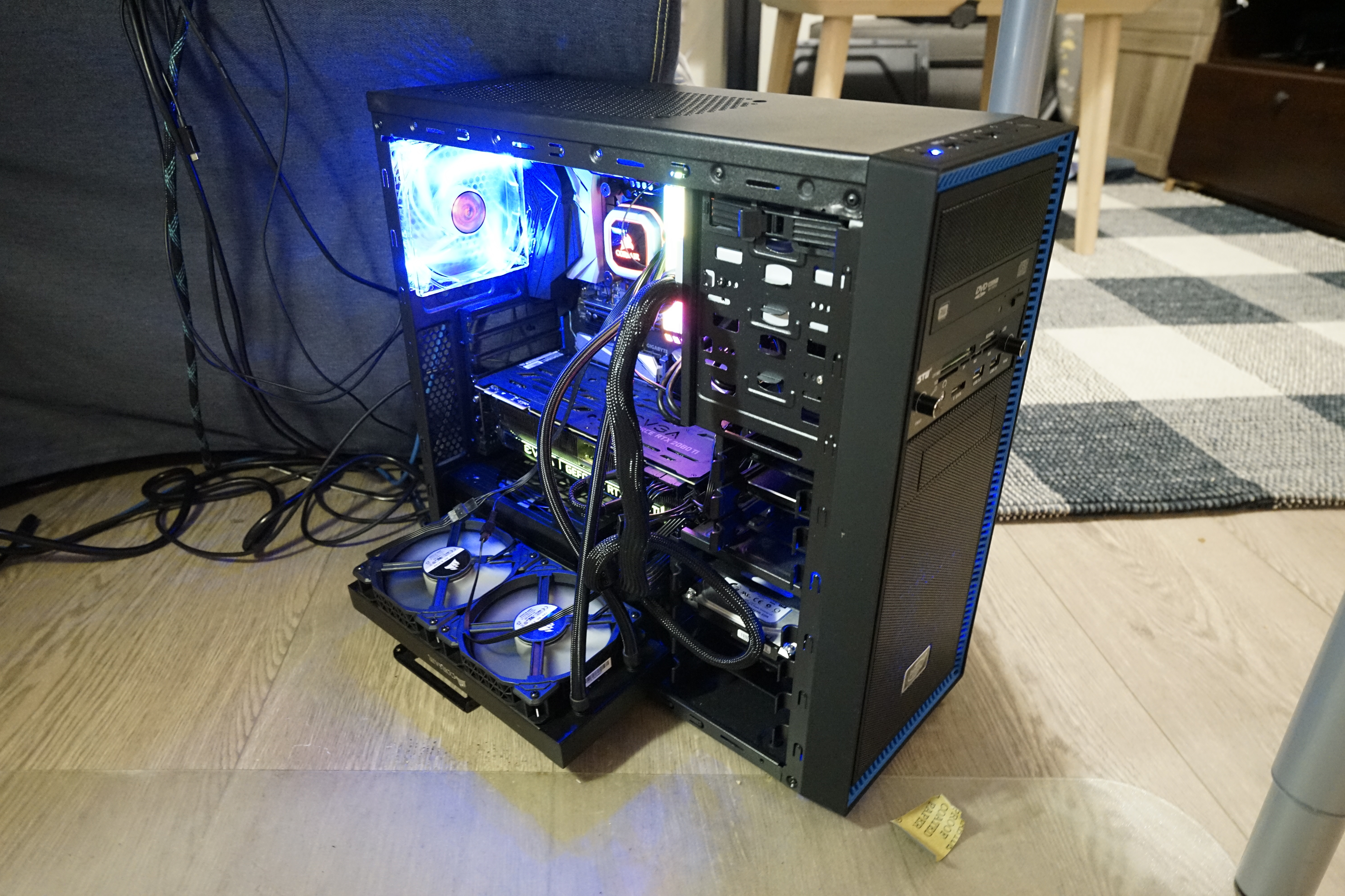
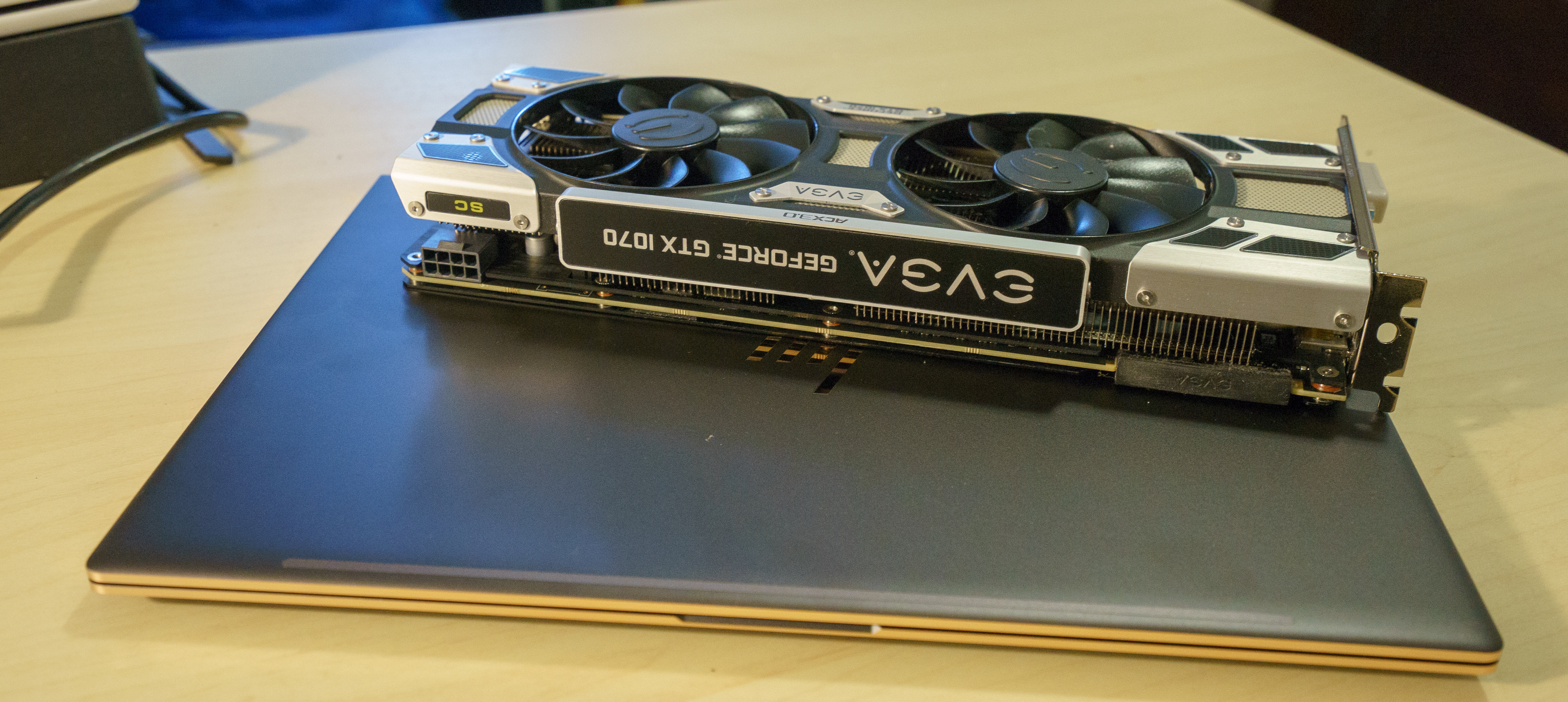
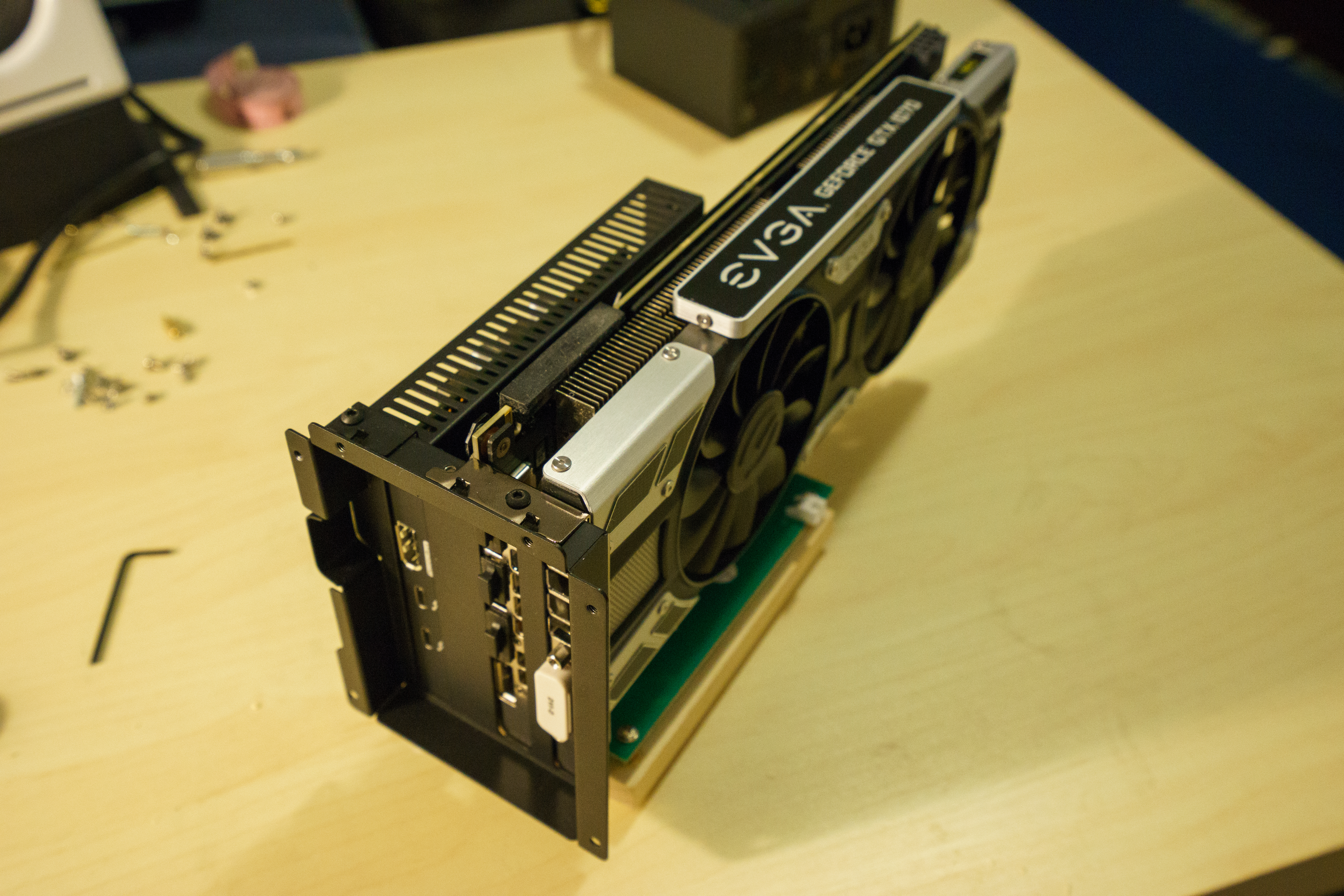
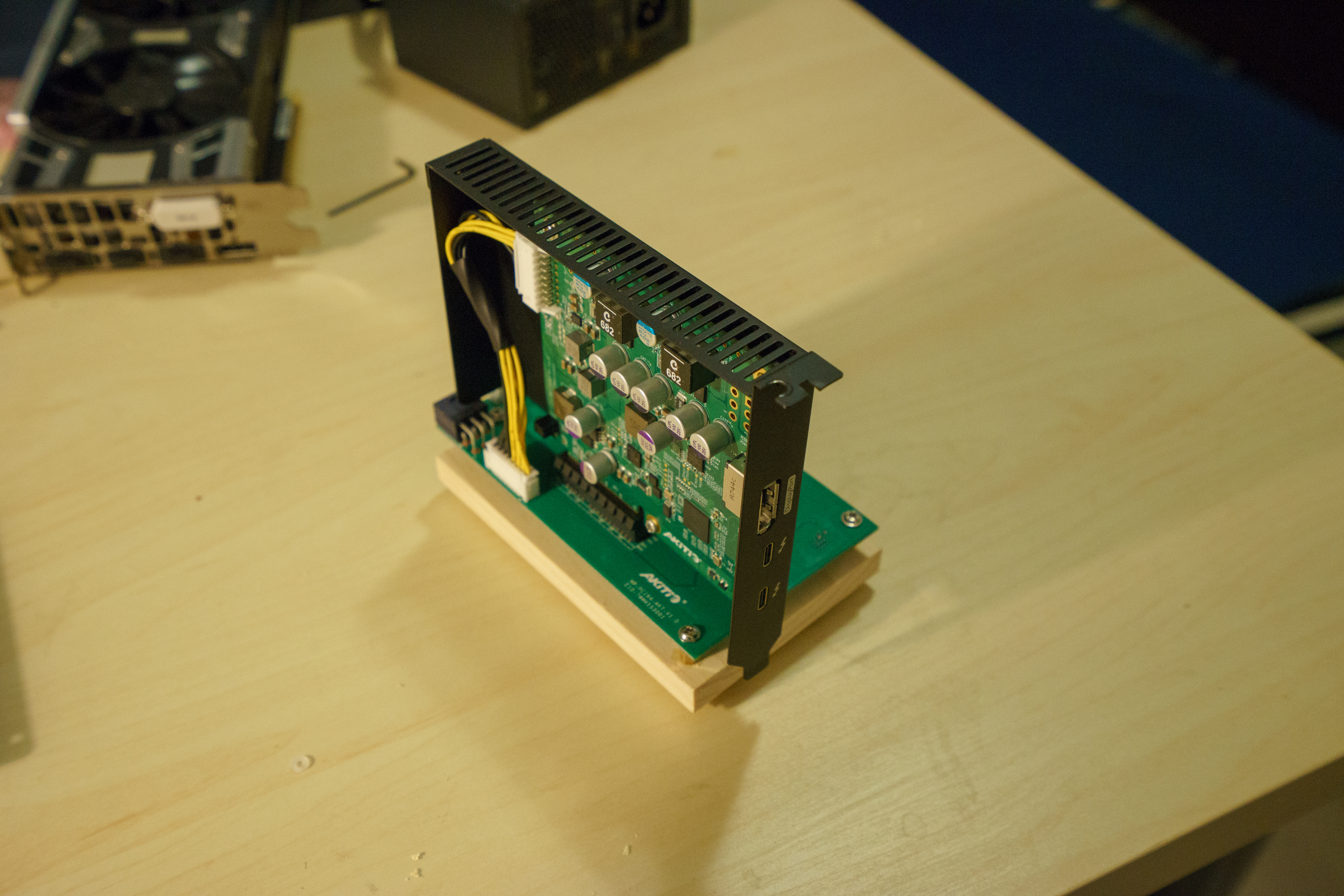
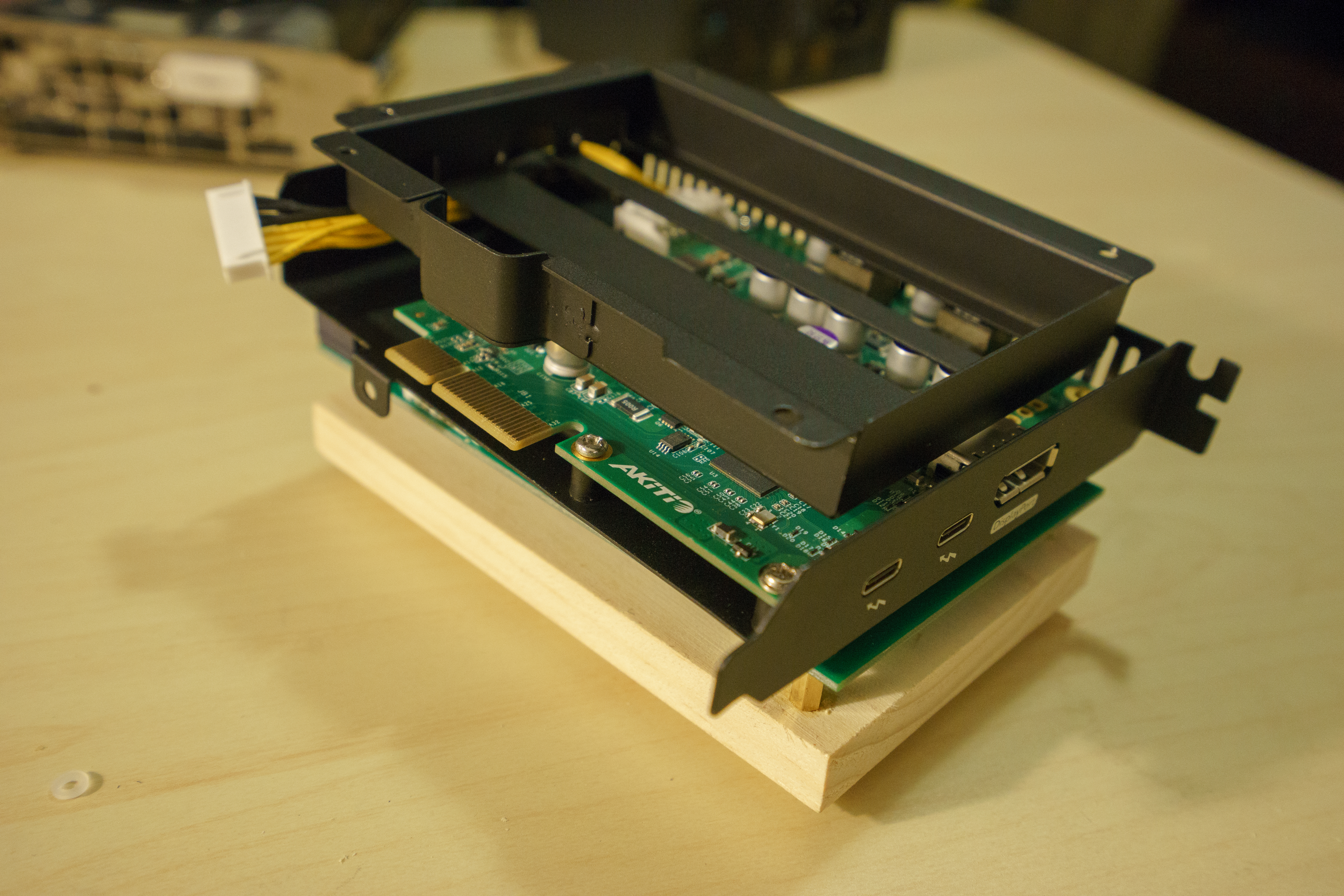
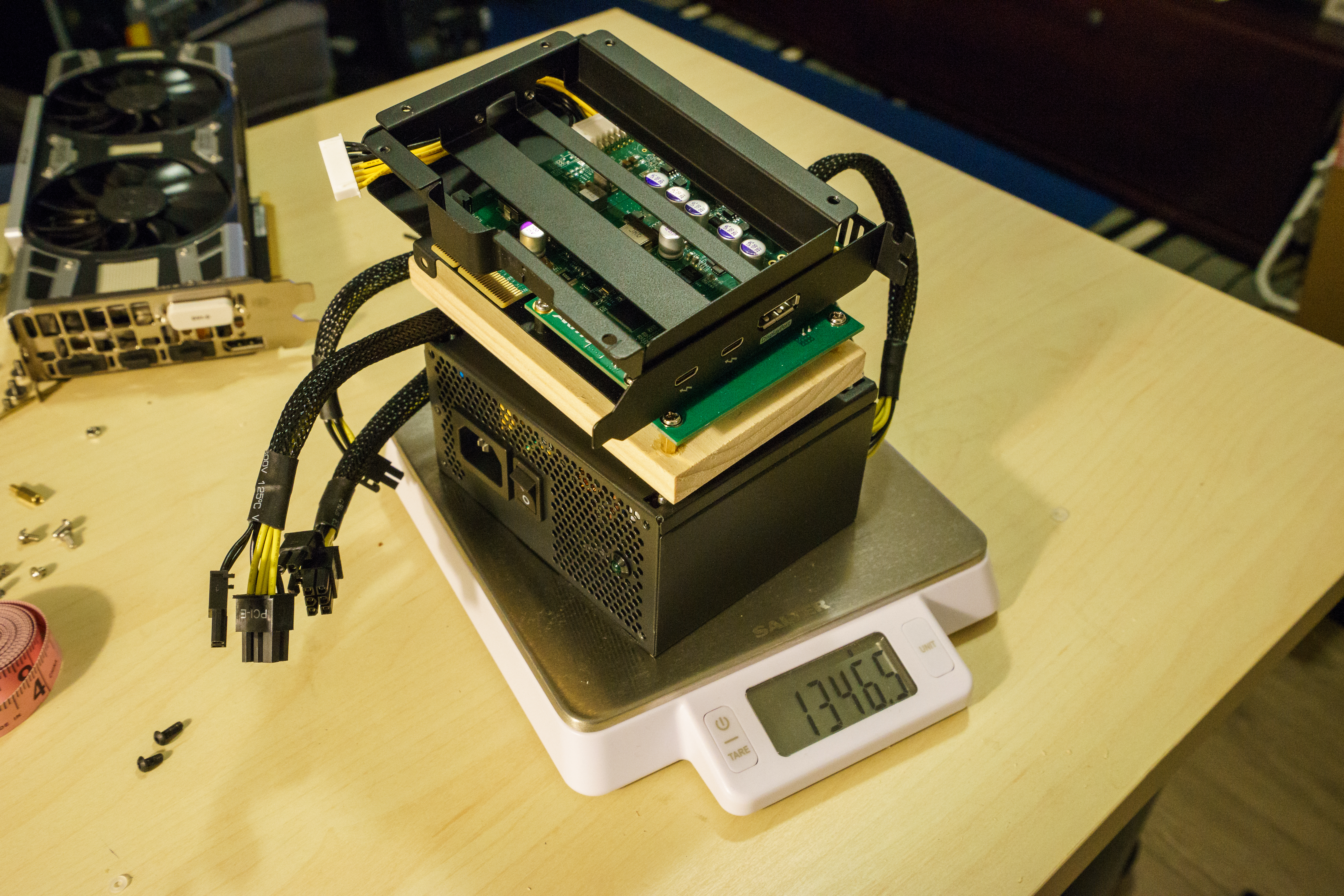
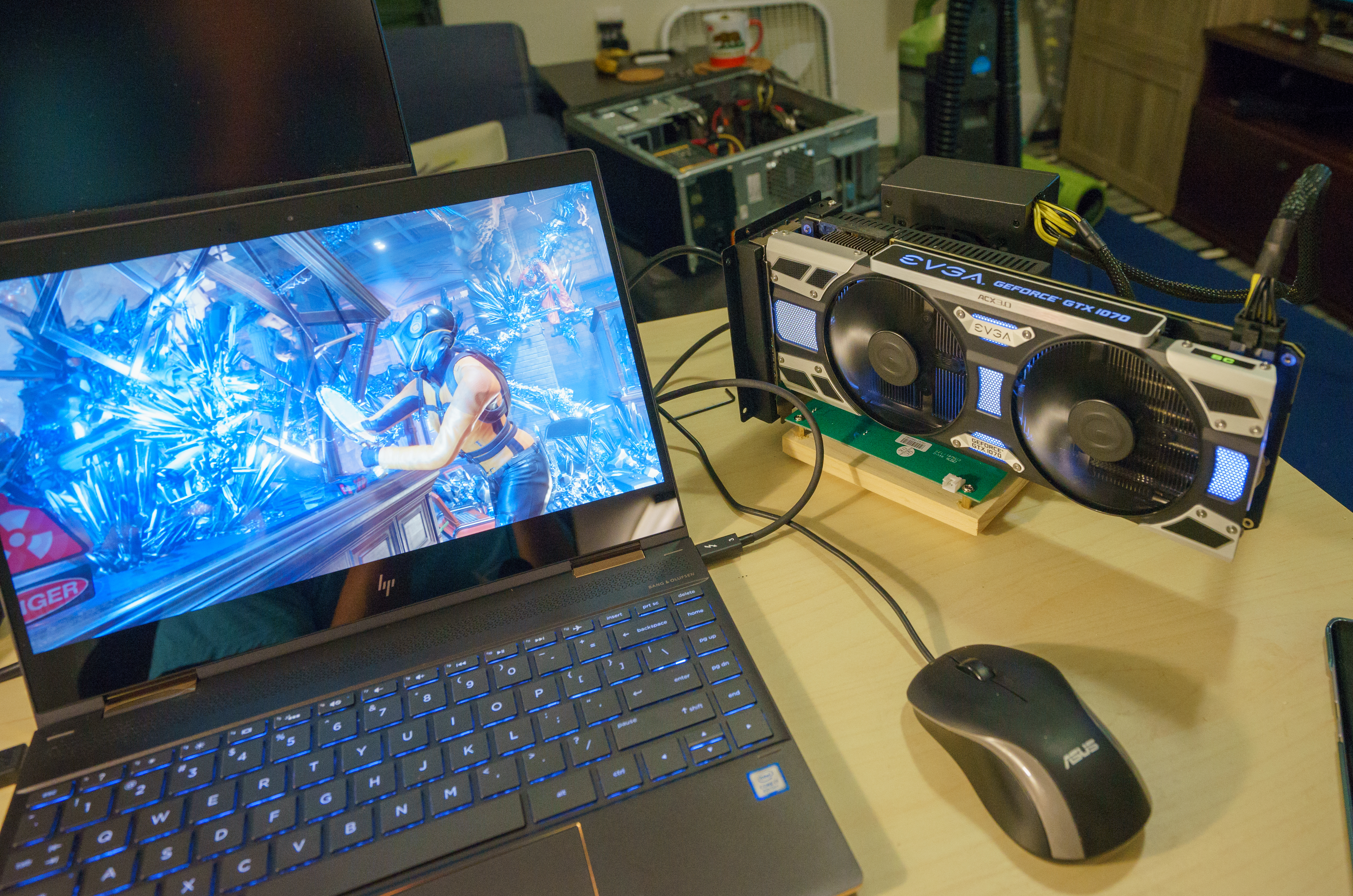
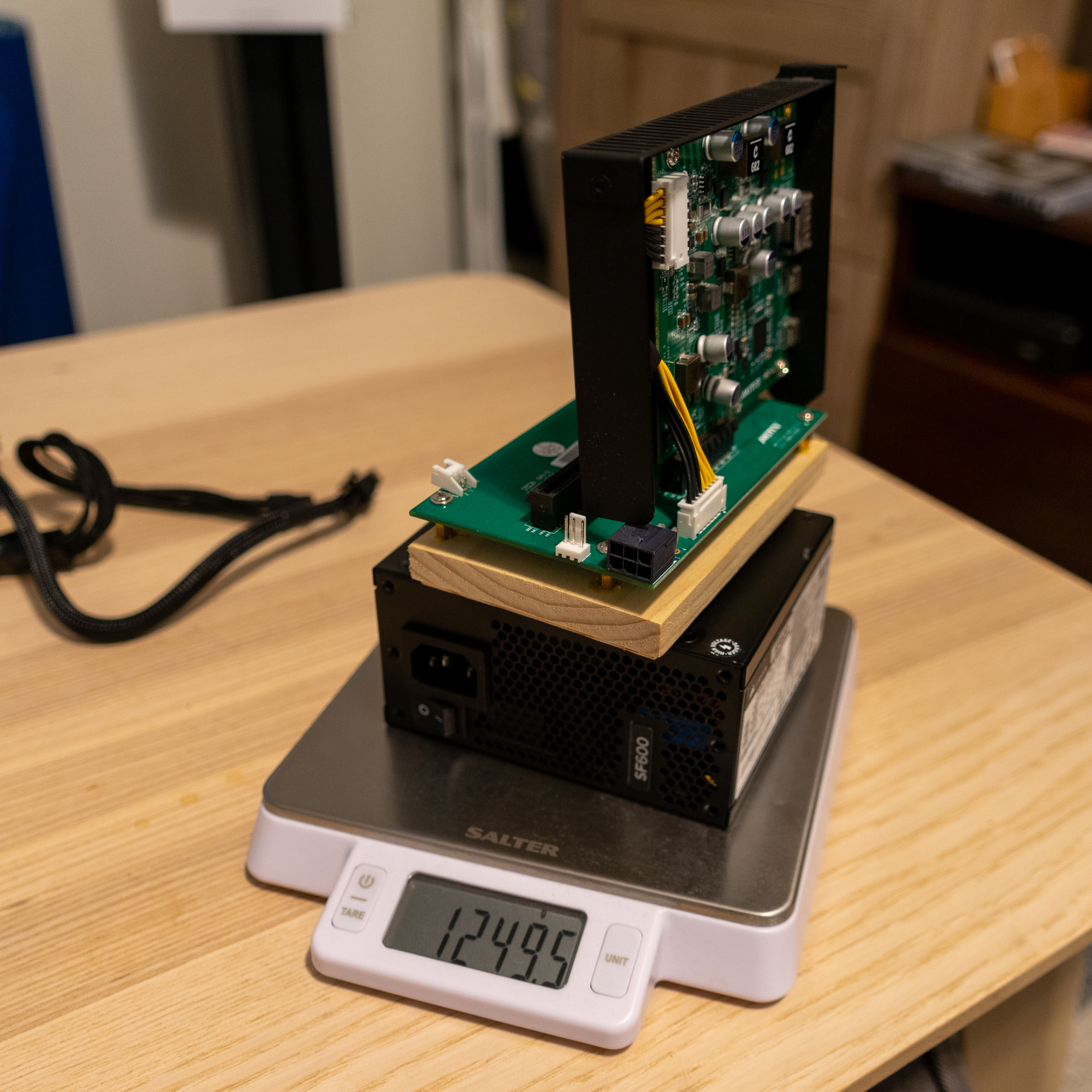
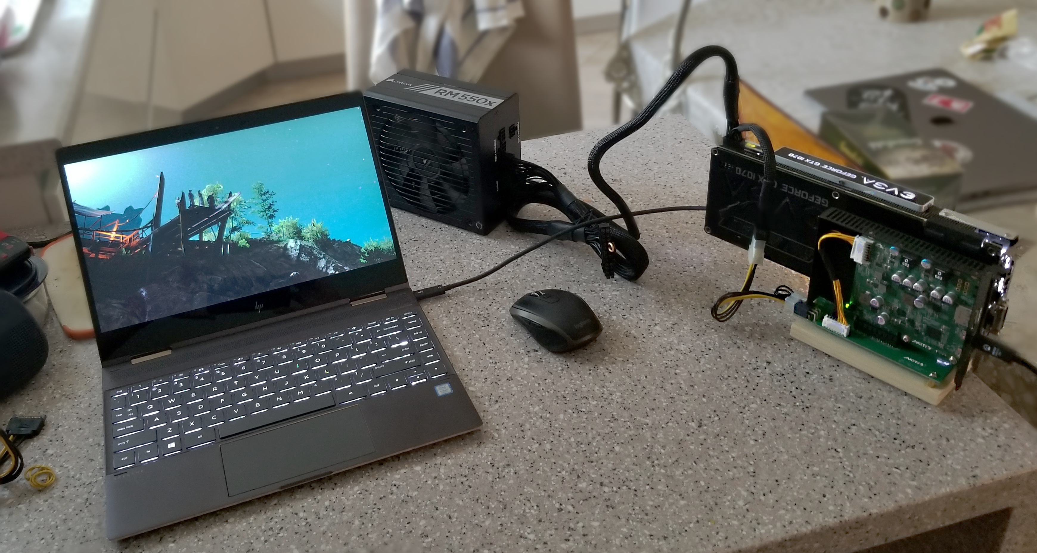
So here it is (without the power supply)

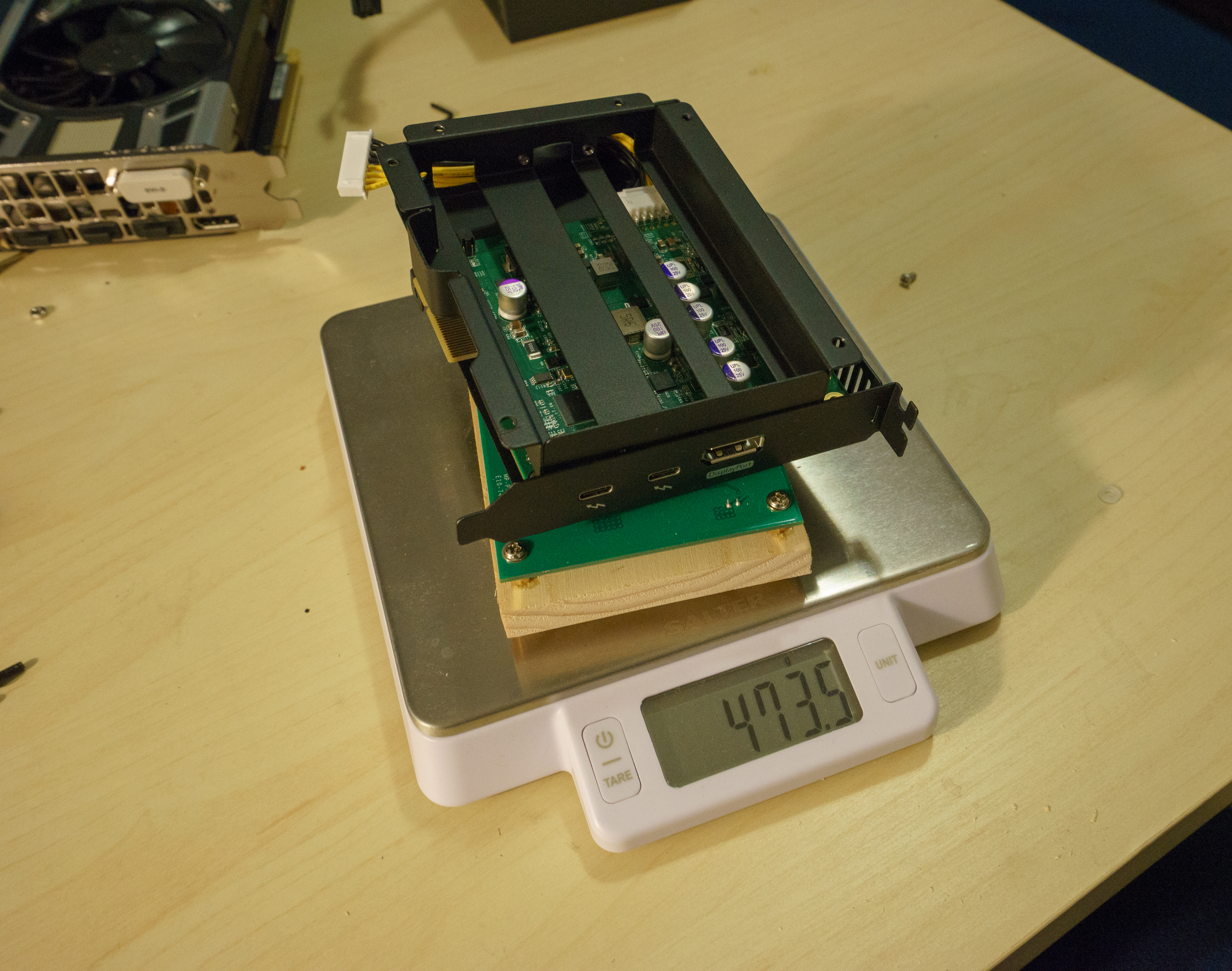
And here it is without the GPU (and without the power supply either)

The final setup weighs just 1.3 kg, including the power supply and 0.47kg without.

In order to improve portability, I only used the X screws when putting things back, and made sure that no T8 or T10 screws are needed, and I can travel with a regular philips screwdriver. Make sure to pick a large enough screwdriver to unscrew that tricky bolt. I tried to use a small screwdriver one might use for watches and I didn’t get enough torque out of it.

Benchmarks

And we’re done. I’ve ran a variety of tests and benchmarks. Note that I ran all benchmarks with the internal display.

3Dmark Time Spy

I ran a 3Dmark Time Spy benchmark multiple times; here are the scores from one run. I also ran it on my PC (same GPU, but a different, older CPU) to check if switching from PC to a Laptop

Test	Score	Percentile	Verdict	Link
Laptop no eGPU	313	bottom 1%		https://www.3dmark.com/3dm/27403962
Laptop with eGPU	3984	better than 40%	top gaming laptop	https://www.3dmark.com/3dm/27403805
Desktop same GPU	5259	better than 47%	what? time to upgrade	https://www.3dmark.com/3dm/27733262

My desktop runs Intel(R) Core(TM) i7-3770, whereas the laptop runs way more modern Core i7-8550U. However, it’s known that CPUs didn’t make much progress in single-core performance over the last several years; most improvements have been in portability and energy efficiency.

Unfortunately, I didn’t use 3dMark Pro, so I couldn’t force 4k for the desktop; it ran under a lower resolution. I suspect, they’d be on par otherwise.

So it seems that the eGPU setup runs as well as the desktop setup with the same GPU (but a way older CPU).

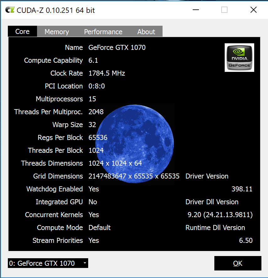
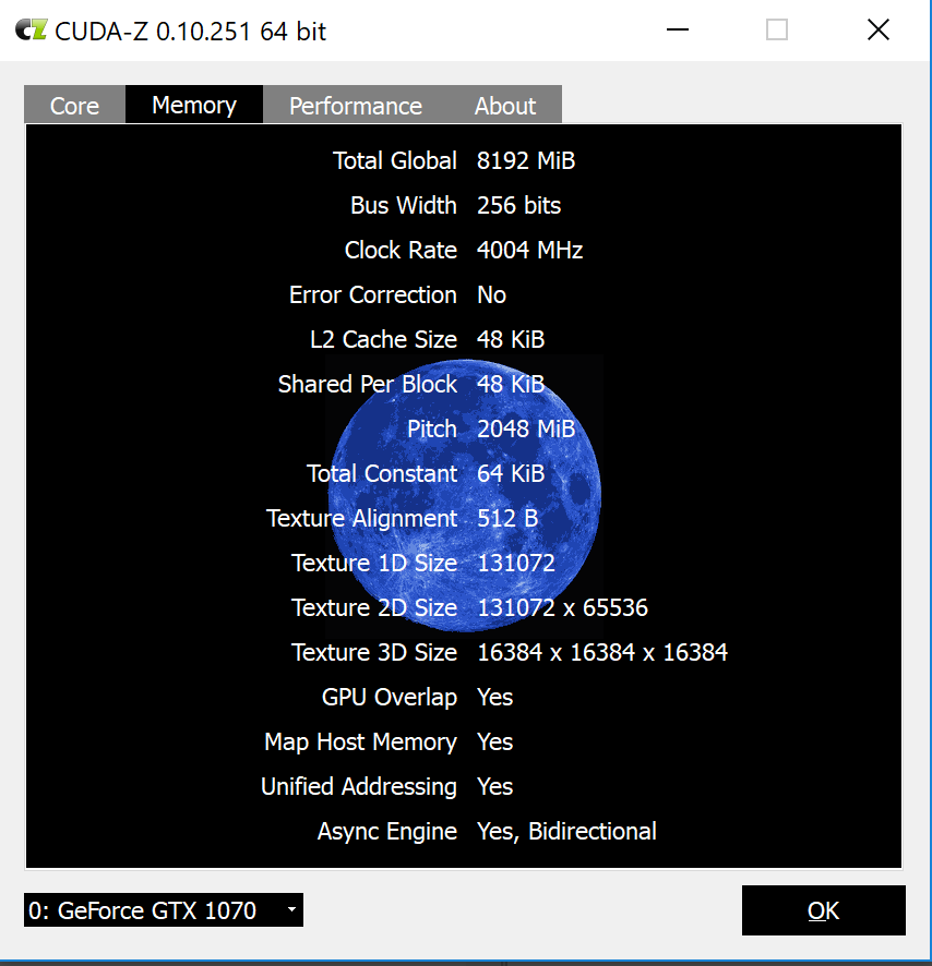
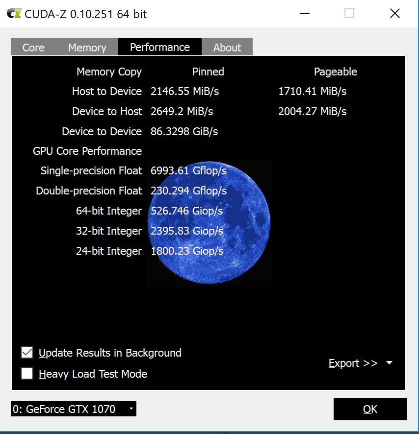
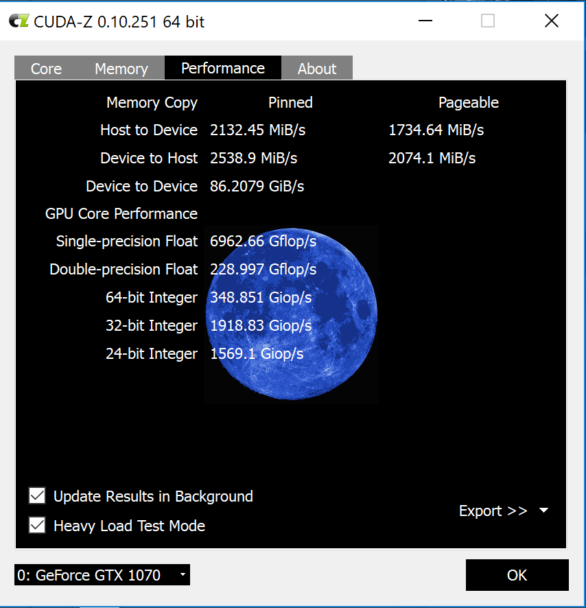
Cuda-Z

I used Cuda-Z software recommended by egpu.io to measure throughput.

It seems, the connection does churn 2Gb/s of data each way, which is good. Overall, I don’t really know how ti interpret the results.

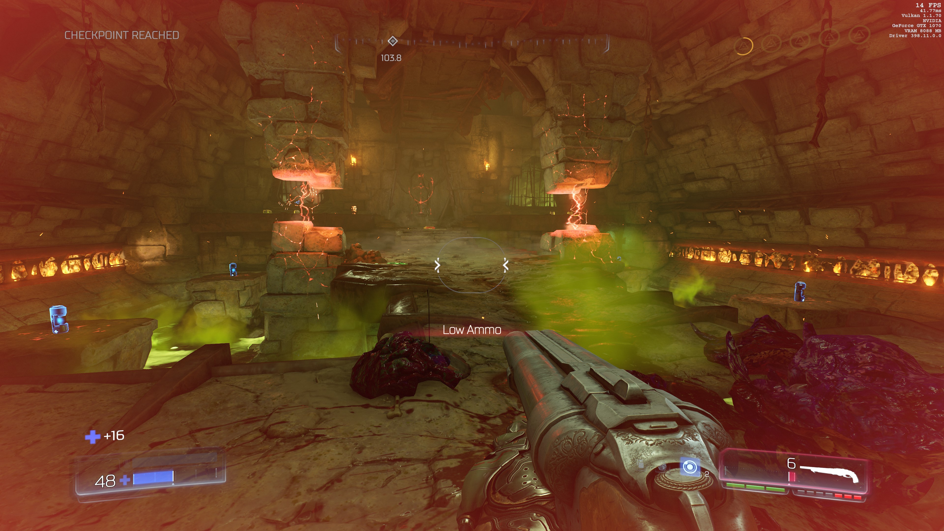
Games

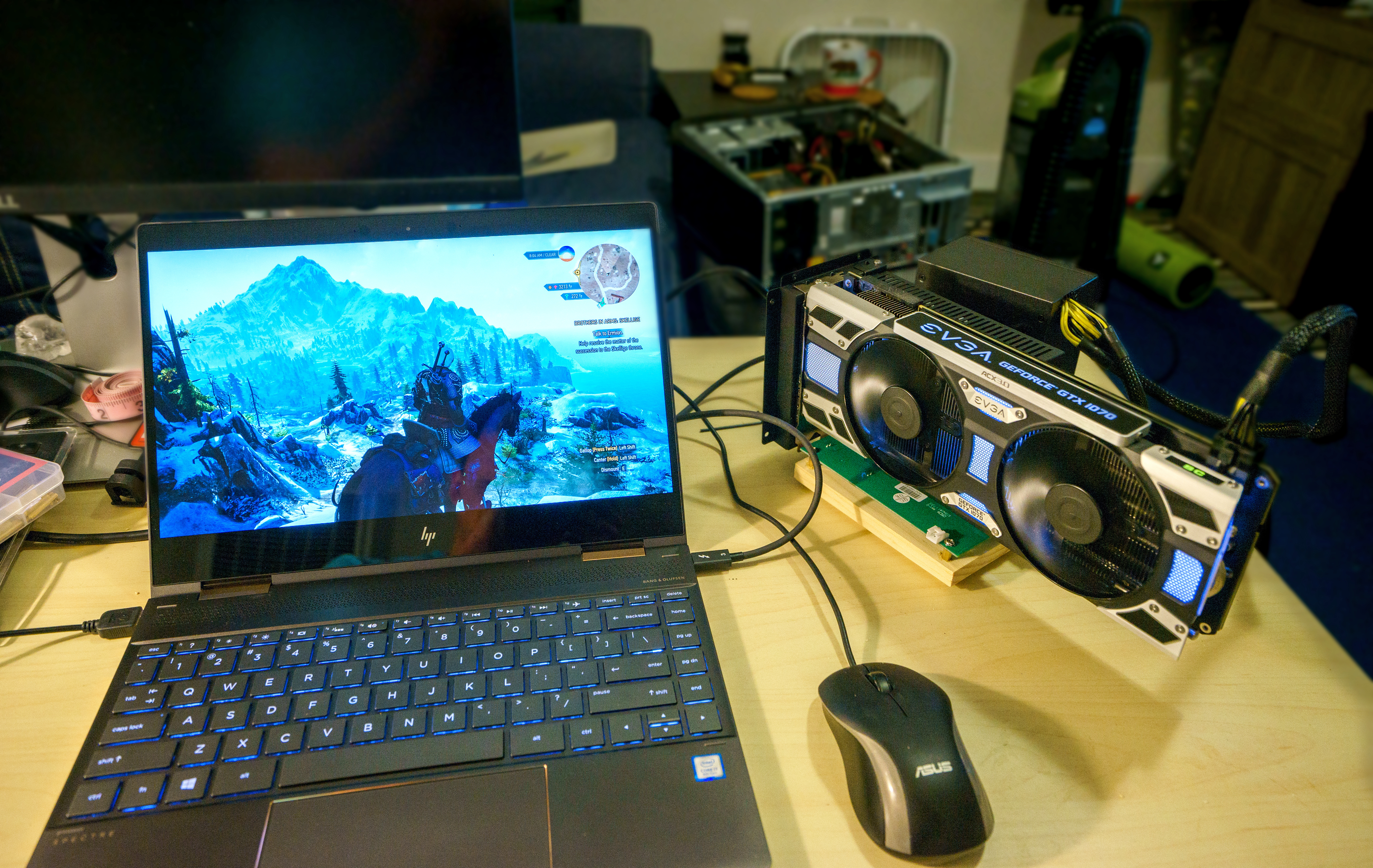
I’ve playes many hours of Witcher 3 (2015) on max settings to great effect. There was no lag, and I enjoyed beautiful and responsive gateway. I also played a bit of DOOM (2016) on Ultra settings, and it was a bit too much (I got 20-30 FPS when walking and most of the fights, but several simultaneous effects lagged a bit). Non-ultra settings were a blast though!

Both games were enjoyed in 4k resolution. It was awesome.

Portability and features

The laptop charges while playing; just make sure to get a 100W-enabled cable.

As an added bonus, Ubuntu Linux 18.04 (bionic) recognized the plugged in video card without any issues or configuration. I haven’t yet tested Machine Learning acceleration but I’ll update this post when I can do it.

Field Test Number one… oops!

How does this setup fare without benchmarks? I was able to get several hours of continous gameplay until the stock Akitio’s power supply died of overheading and never recovered. The boards, the GPU, and the laptop were OK, but the power supply just stopped working.

I can’t quite tell what prompted it, but I did notice that the fan didn’t turn on. It used to but it didn’t. I must have damaged the unit when transporting it in the checked in luggage (or maybe it was just garbage to begin with).

Common ATX Power Supply Replacement

This section is probably not interesting to you as I’m unsure your power supply will blow up. So please skip to the final Field Test section.

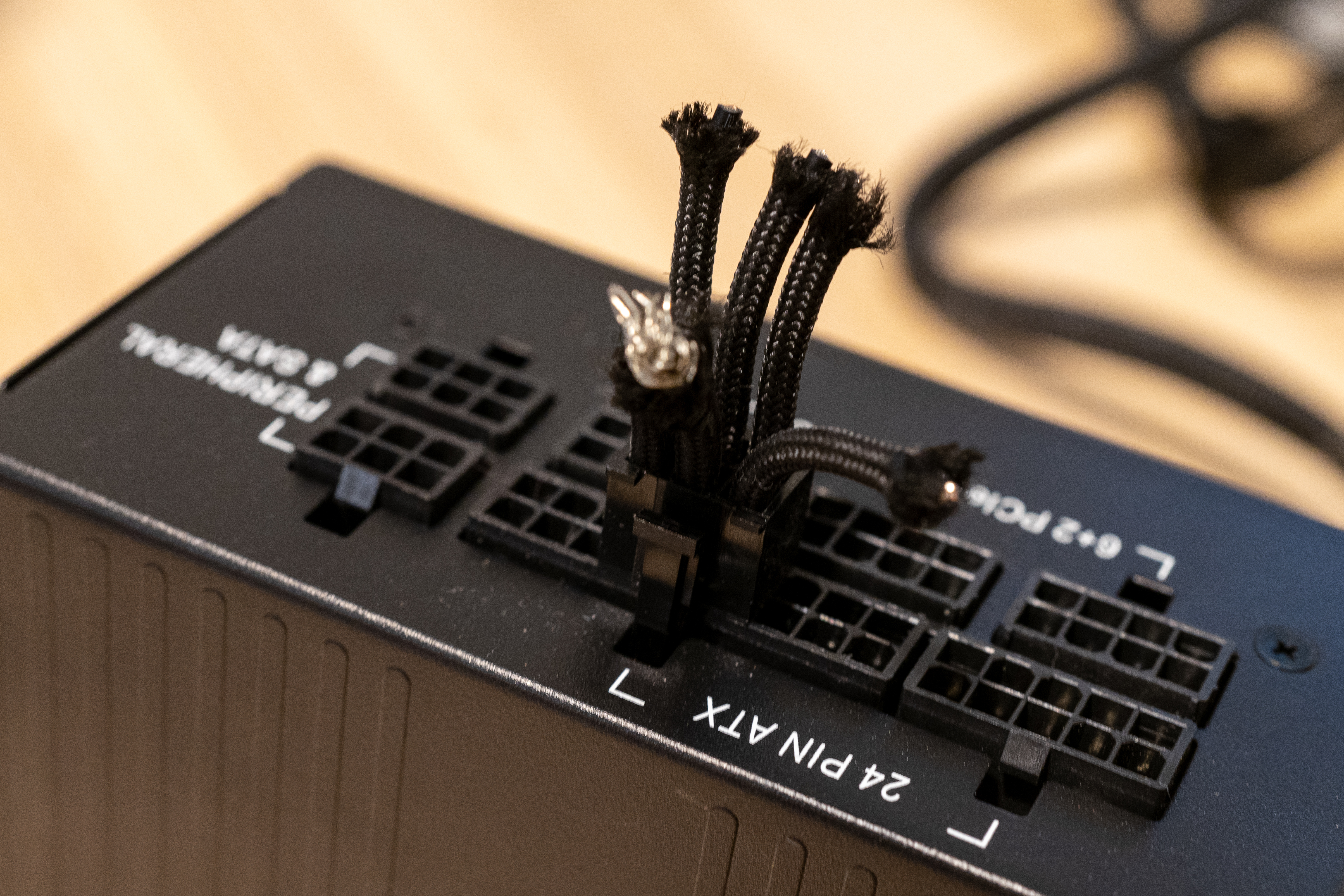
Instead of trying to recover, debug, and fix the dead power supply, I just bought a new one. I immediately noticed the difference between the Akitio’s power supply and the typical ATX power unit.

1. Akitio’s Power Supply is smaller than many standard ATX units and it weighs less (0.8 kg vs 1.5kg)
2. …it only has PCI-E cords whereas ATX has all of them
3. …it has two PCI-E power connectors, but they are on different wires. The ATX power supply I got has two of them attached to the same wire, and the distance between them is quite short!
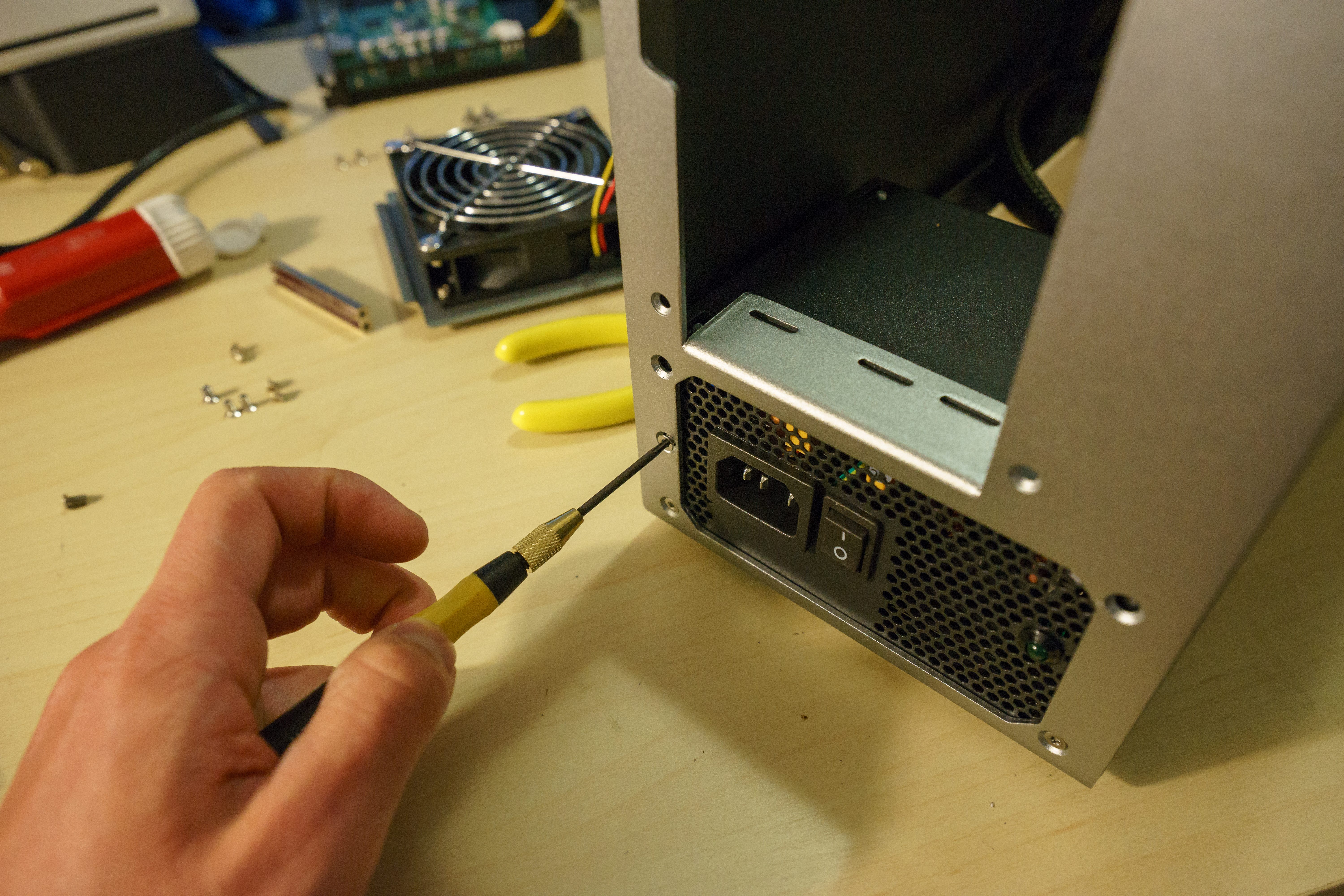
4. …it turns on when the switch on the back is flipped, whereas a normal ATX power supply requires another switch to power-up, which motherboards usually supply but we don’t yet have.

In 2018, when the post was originally written, I’ve replaced the original PSU with a Corsair 550W modular supply RM550x which I wouldn’t do now. Its main feature was modular wiring so that the extra wires could be discarded, and that’s what it looked like.

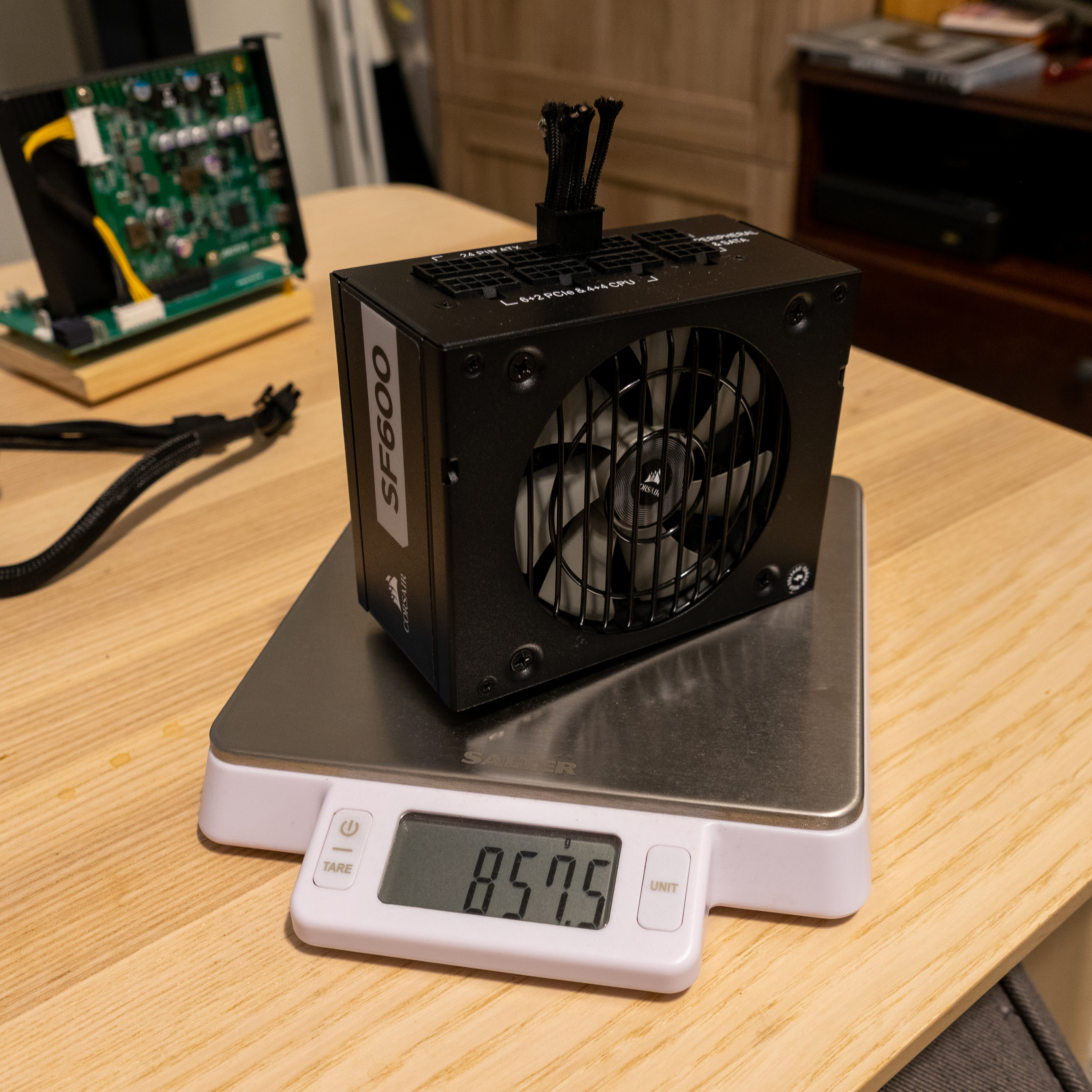
Later, I’ve purchased a more compact Corsair SF600 that weighs half as much as RM550x, and is thus similar to the original Akitio PSU. The entire setup is now back to 1.3 kg again.

Since the ATX power supply requires the user to press a power-on button, you need to emulate it as if it’s always pressed. You do this by short-circuiting the pins that are normally connected to the power on button via the motherboard. That way, the PSU will start powering the GPU when you press the on/off switch on the PSU itself.

I googled the pin layout for my PSU, cut the wires from one of the spare connectors and short-circuited the power on pins like so:

This plug simply sits there at all times; there’s no need to unplug or replug it. Also, the pin shapes didn’t exactly match, but with enough force, any connector can be plugged into any slot 🤓.

Wi-fi Interference testing

I heard, the major reason Thunderbolt 3 eGPUs come with a huge enclosure is to prevent the electromagnetic field emissions. Supposedly, Thunderbolt 3 boards emit quite a bit of EMF radiation, and this can cause Wi-fi interference.

I wasn’t able to find the evidence of that. I measured wi-fi connectivity speeds and signal strength and I wasn’t able to notice a drop. That doesn’t mean there was no packet drop: perhaps, the wi-fi connection was indeed broken, but my 100Mb/s broadband was too slow to actually affect the speeds. It also could be that you’d need say 5 Thunderbolt 3 cards to emit enough EMF.

I used my cell phone to measure signal strength and used OOKLA speedtest to measure up- and download speeds. I placed cell phone into three places: 2ft from Wi-fi router, 12 ft from Wi-fi router, and into the other room. I also placed eGPU into three positions: 2ft from Wi-fi router, 10 ft from Wi-fi router, and completely off. Here’s what it looked like when the eGPU is 2ft away from Wi-fi; you can see the Ubiquiti wi-fi “White Plate” in the top right corner:

I was running the Unigine Superposition benchmarks while measuring the signal strength and the download speeds, in case the EMF interference only appears under load.

Science log is here. The results are in the table below, each cell contains “Download speed (Mb/s) / Upload Speed (Mb/s) / Signal Strength (db)".

So this means my Wi-fi stays pretty much unaffected regardless of eGPU presence. If there was packet drop, it didn’t affect the 100 Mb/s connection.

Optional Addons

Buy a longer USB3 Thunderbolt-enabled cable ⚡

The USB cable that comes with the Akitio Node Pro is quite good but a bit too short. No wonder: a longer cable will cost you. A detachable cable that affords the required throughput needs to conform to som Thunderbolt 3 standard, and support 40Gbps data throughput. I simply bought a pretty long, 6ft cable by Akitio hoping for best compatibility, and I’ve had no issues with it. The Field Tests were done on that longer cable.

Putting the enclosure away reduces noise and improves mobility: you can put the setup close to the power outlet and attach to it from a different side of the table.

Use that extra fan

Akitio Node Pro had one extra fan to draw air into the case, and it is now unused.

Optionally, you can attach it to the board where it originally was. If I were to do this, I would also screw some leftover standoffs into the fan so it gets better intake. The original case had a curve to separate it from the ground. However, I got good enough performance out of the video card.

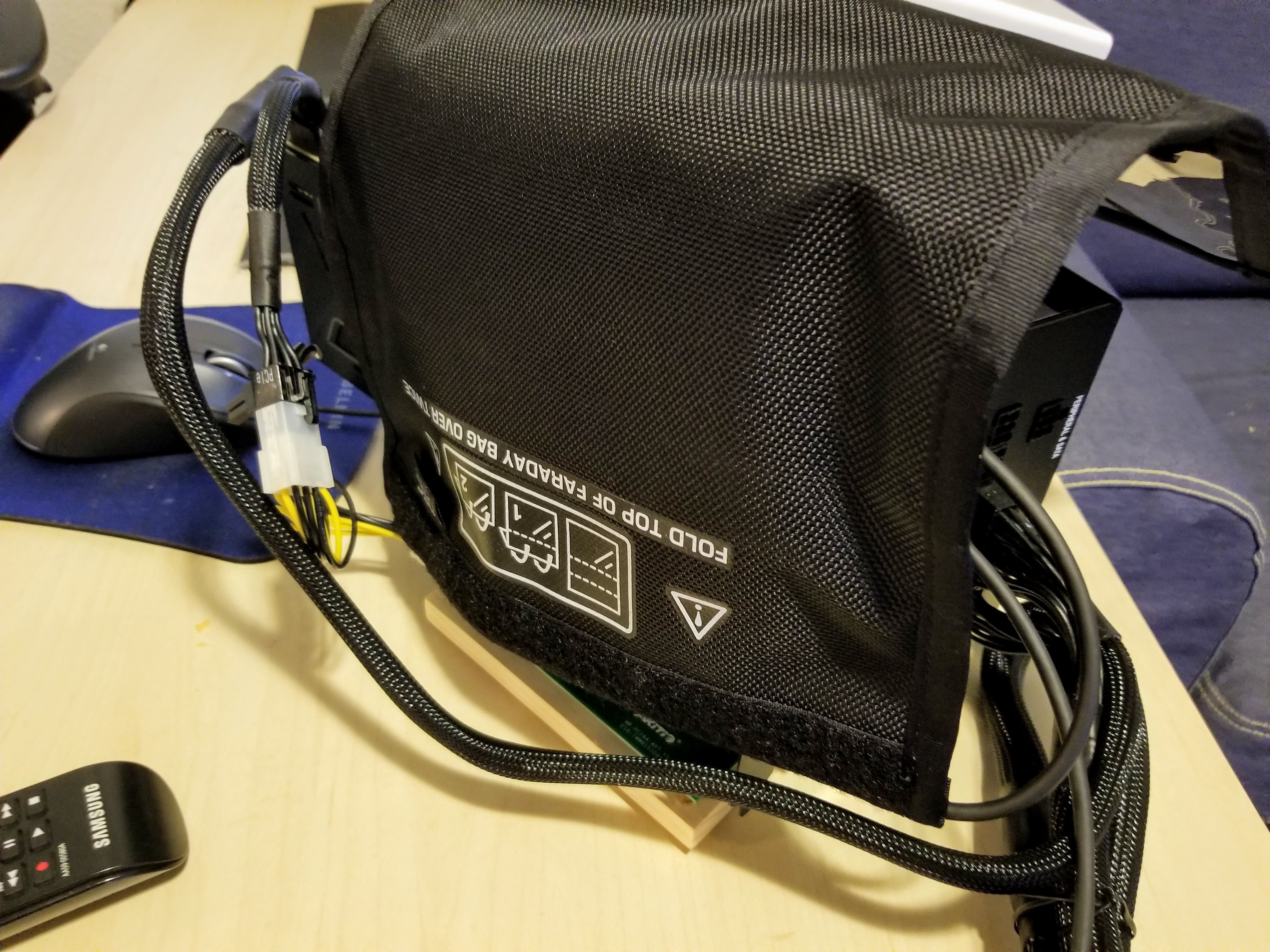
Faraday Bag

A way to reduce EMF exposure is to put the emitter into a Faraday Cage or a special bag.

This one actually works. As probably do others, but just a month ago there used to be many scams on Amazon of faraday cages that you should place on top of your router, and they would “block EMF”, improve your health, and make Wi-fi faster at the same time. 😂 This Farady bag actually works (I tested it by placing a cell phone and calling it to no avail). I can’t tell you have to use it, but maybe it could put your mind at ease.

Final Evaluation and notes on performance

It works. Moreover, the power supply doesn’t overheat. I have never seen its fan turn on. Perhaps, the larger size allowed to space the internals better, or perhaps it’s just of better quality.

The performance is stellar, even with the internal display. Various measurements (done by other people) detect that using the internal display on a laptop or connecting an external display to the laptop (as opposed to connecting it to the video card itself) saturates some bottleneck and results in a performance drop. My findings are consistent with this blog post on egpu.io: with a card like GTX 1070, you won’t notice the drop because you’re getting 40+ FPS anyway.

After playing Witcher 3 at “Ultra High” quality (!), with full-screen antialiasing (!!), at 4k resolution (!!!), for several hours (was hard to resist anyway), I am happy to call it a success.

Moreover, the setup survived a transcontinental flight in the checked-in luggage, wrapped in underwear and padded with socks. And now, just one challenge remains: get it through TSA in a carry-on and prove the bunch of wires is a gaming device.

In the previos post, I described why I chose Amazon AWS elastic Beanstalk for this blog. AWS Elastic Beanstalk (EBS) is the way to deploy Docker containers on the autoscaled Amazon Cloud with zero setup. It’s similar to App Engine Flexible Environment, but slower and harder to use. But how do you actually use it?

This post contains a speed run of setting up AWS Elastic Beanstalk. It’s easy to lose your way in AWS documentation, and I hope I can make it easy for you here.

We’re going to set up a very simple application, that has only 1 type of instances. In my case, this instance serves 1 docker image with a simple web server listening to port 80. Hopefully, when this guide becomes popular, the instace will scale up (wow!). Otherwise it will just be the cheapest thing AWS can do for some simple custom code with no disk or mutable state (aka a database).

Choose the right product (which is “Elastic Beanstalk”)

The first challenge is to not confuse it with other, less useful Amazon products. It’s harder than it seems. You do not want Amazon Elastic Container Service despite that it has the word “Container” in it, but “Elastic Beanstalk” only seems to offer beans, or stalking or both. The “Container Service” is a counterpart of EBS that requries you to set everything up manually, including your Elastic Private Network, Managed Instance Group, Elastic Load Balancer, and other Crap You Don’t Care about. On top of that, you will have to manually update Docker installations. “So uncivilized”.

Configure private Docker Registry

The next challenge is, find out a way to deploy Docker containers to your private repo. You need Amazon Elastic Container Registry (this one both has the word “Container” and is actually useful). Create a repo for your server image (let’s call it megaserver). Optionally (later), add a “Lifecycle Policy” that deletes old images automatically. But for now, you need to configure the client.

Click on “View Push Commands”, which will show you something like this:

aws ecr get-login --no-include-email --region us-west-2

and it will direct you to AWS command-line client installation guide.

Create the Elastic Beanstalk app

Go to the Elastic Beanstalk, and click “Create New Application” in the top right corner. Choose some sensible name; it doesn’t matter. Then, inside the application, choose “Actions”, then “Create new environment”. Choose “Docker” as the platform.

Now, deploy your first version. Download and configure the eb app, which orchestrates deployment of your local docker images to Elastic Beanstalk. Follow the AWS-supplied user guide–Just substitute PHP they use as example for “Docker”. Also skip the DB if you don’t need one, like I didn’t. Run the eb init, and follow this guide to configure Access Keys.

sudo apt-get install -y python-dev python-pip && sudo pip install awsebcli
eb init

If eb init shows some permission error, try enabling AWSElasticBeanstalkFullAccess permission.

Make sure that your ~/.aws folder did not exist before running these commands! If you were playing with other AWS products, you might have already written something there and corrupted it somehow. So if some auth commands don’t work, try removing the folder and then running:

rm -r ~/.aws
eb init
$(aws ecr get-login)

(The last line means “run aws ecr get-login, then run the command it printed to the console. It prints a docker login command that would authorize docker push to put containers to the AWS registry. )

Now, your keys should be in ~/.aws/credentials. Mine looks like this:

[default]
aws_access_key_id = ASDFKGEWOFKWEOCWCEWOJ
aws_secret_access_key = BoopBoop12345/+/BlahBlahBlahfoobar

As part of the Beanstalk Command-line tool workflow, you’ll need to create ebs/Dockerrun.aws.json in your working folder. See here for documentation. Here’s the file I created (note how it uses the image repository name megaserver we created above).

{
  "AWSEBDockerrunVersion": "1",
  "Image": {
    "Name": "12345567890.dkr.ecr.us-west-2.amazonaws.com/megaserver",
    "Update": "true"
  },
  "Ports": [
    {
      "ContainerPort": "80"
    }
  ],
  "Volumes": [],
  "Logging": "/var/log/nginx"
}

Now, you can finally deploy your image:

docker tag boring_volhard 12345567890.dkr.ecr.us-west-2.amazonaws.com/megaserver:latest
docker push 12345567890.dkr.ecr.us-west-2.amazonaws.com/megaserver:latest
eb deploy --verbose

If all the permission are correct, your image will start deploying, and will be available within 1-2 minutes.

Update the application

When you want to deploy the next version, just repeat the same commands. You’ll see how the image is being updated on the environment page.

docker tag boring_volhard 12345567890.dkr.ecr.us-west-2.amazonaws.com/megaserver:latest
docker push 12345567890.dkr.ecr.us-west-2.amazonaws.com/megaserver:latest
eb deploy --verbose

If you set the Environment parameters correctly (I don’t remember if you need to change the defaults or not), it will perform a rolling update, where it would replace your running containers one-by-one.

Here’s the configuration that works for me. Note the “Rolling updates and deployments” in the middle. This website can scale to more instances based on network I/O (particularly, based on the O).

Keep the change

My bill for one micro instance is $0.85 per day, which brings it to… $26 a month. In a quirk of Amazon Billing, it says I’m paying the most (65%) for the Load Balancer rather than for “running the instances” (27%). Based on which, it seems to me, these costs are made up anyway. Consider this the minimum price at which one can run AWS beanstalk with dockers.

Here’s the resultant cost profile.

Overall, this setup worked for my blog. I hope it works for you as well.